Structural dynamic factor models
Session 10 · Lecture notes
The BSE monetary-policy exercise estimates static factors by principal components, fits their VAR, and retains four dynamic innovation directions. I distinguish the retained-rank covariance from the full covariance, derive the observable recursive identification, and make the policy-shock normalization explicit. A separate scalar Kalman-filter example explains the treatment of missing measurements without presenting it as an empirical state-space replication.
1 Static factors and dynamic shocks
A panel may require several factors to describe its contemporaneous covariance even when a smaller number of economic disturbances drives their dynamics. A static factor dimension counts the coordinates needed to represent the common component. A dynamic shock dimension counts independent innovations. They need not be equal.
The BSE US monetary-policy exercise estimates a structural dynamic factor model by principal components and a factor VAR. It follows the structural factor approach of Forni and Gambetti (2010), but uses a different quarterly classroom dataset. It is not a maximum-likelihood state-space or EM replication. I keep that distinction explicit, then introduce a separate known-parameter Kalman-filter example to connect this chapter with the nowcasting notes.
The prerequisites are Session 09’s principal components, the VAR moving-average representation, and recursive identification. The central calculation here is a low-rank approximation to the factor innovation covariance. The exercises check its dimensions, the variance it discards, the monetary-policy normalization, and the behavior of a filter when a measurement is missing.
2 The classroom data
factor_data.mat contains an already transformed panel, column names, and transformation codes. Its observed dimensions are 242 quarters by 210 series. It contains no date vector. The calendar 1959 Q3 through 2019 Q4 is asserted from the original script and checked against the row count; it is not inferred from raw observations in the MAT file. The saved result records this limitation in data.calendarSource.
The input fingerprint is essential because a different 242-row panel could have different dates. There is also no claim here to have rebuilt the source transformations from raw FRED series: only the transformed classroom vintage is available in this input. No additional differencing or missing-data imputation is performed before factor estimation.
The original MATLAB file, lecture PDF, and several comments disagree about factor selection and dimensions. The executable file selects Bai-Ng IC2 among one through twenty static factors. On these bytes it selects seven factors, not the ten-factor example described in the lecture PDF. The code fixes four dynamic shocks after computing other diagnostics. This replication follows those actual assignments and does not rerun unused ABC or Hallin-Liska diagnostics.
3 Choosing the static dimension
After standardizing each transformed series, let Z be the resulting T\times N panel. For each candidate r, principal components give a common component \widehat F_r\widehat\Lambda_r' and residual variance
V(r)=\frac{1}{NT}\left\|Z- \widehat F_r\widehat\Lambda_r'\right\|_F^2.
The implemented information criterion is
IC_2(r)=\log V(r)+r\frac{N+T}{NT}\log\{\min(N,T)\}.
The first term rewards approximation accuracy; the second penalizes additional factors as a function of both panel dimensions. This is one criterion from Bai and Ng (2002), not a likelihood-ratio test. Its minimum is stored alongside every candidate objective so the selected count can be checked directly.
With seven static factors, the code estimates a factor VAR with an intercept and selects one quarterly lag by the classroom BIC convention. The empirical factor scores and loading vectors retain the same unit-length-loading normalization as Session 09. Full-sample standardization is used for this historical exercise, not for a real-time forecast evaluation.
4 Reducing innovation rank
Write the factor VAR innovations as \varepsilon_t with estimated covariance \Sigma_F, an r\times r matrix. Let
\Sigma_F=K_{all}\operatorname{diag}(d_1,\ldots,d_r)K_{all}', \qquad d_1\geq\cdots\geq d_r\geq0.
Keep the first q=4 eigenvectors in K_q and set M_q=\operatorname{diag}(\sqrt{d_1},\ldots,\sqrt{d_q}). The reduced-rank impact matrix is R=K_qM_q, with dimensions r\times q. Its covariance is
RR'=\sum_{j=1}^{q}d_jk_jk_j'.
This equals the full \Sigma_F only when all discarded eigenvalues are zero. The classroom discussion sometimes writes a full-covariance equality after truncation; that equality does not hold for a positive discarded spectrum. The result therefore reports both the full eigenvalues and the retained trace share \sum_{j=1}^{q}d_j/\sum_{j=1}^{r}d_j. Here the four-shock approximation retains about 88.29 percent of factor-innovation variance. It does not retain 88.29 percent of every observed series’ variance.
The projected shocks
w_t=M_q^{-1}K_q'\varepsilon_t
have identity covariance under the same residual covariance divisor. The code uses a diagonal linear solve for this operation. Reconstructing Rw_t gives only the innovation component in the retained eigenspace, not all of \varepsilon_t.
5 Identifying monetary policy
Let C_h denote the r\times r factor-VAR moving-average coefficient, and let D_s contain the original series standard deviations. The unidentified observed-panel response is
B_h=D_s\widehat\Lambda C_hK_qM_q,
with dimensions N\times q. Multiplying by D_s restores transformed observed-series units after PCA standardization. It does not add a response from the idiosyncratic component, which remains outside this structural common-component calculation.
Select the impact rows for GDP, CPI, the federal funds rate, and the EXSZUSx exchange-rate series in that order. Their q\times q block is B_0^m. As in Session 09, solve
H=(B_0^m)^{-1}\operatorname{chol}(B_0^m B_0^{m'}),
using the lower Cholesky factor. The rotation is orthogonal, and B_hH gives structural responses. The third shock is the monetary-policy shock: GDP and CPI have zero impact responses, while the exchange-rate series may move immediately. Those zeros are identifying assumptions about the common components of the transformed observables.
For reporting, only the third shock column is rescaled so that its federal-funds-rate impact is 0.5 percentage points, or fifty basis points. The underlying unitShocks retain unit covariance; policyScale records the separate response normalization. The source multiplies every shock column by the policy scale. That is unnecessary for the policy figure and obscures the interpretation of the other shocks, so I do not retain it in the preferred result.
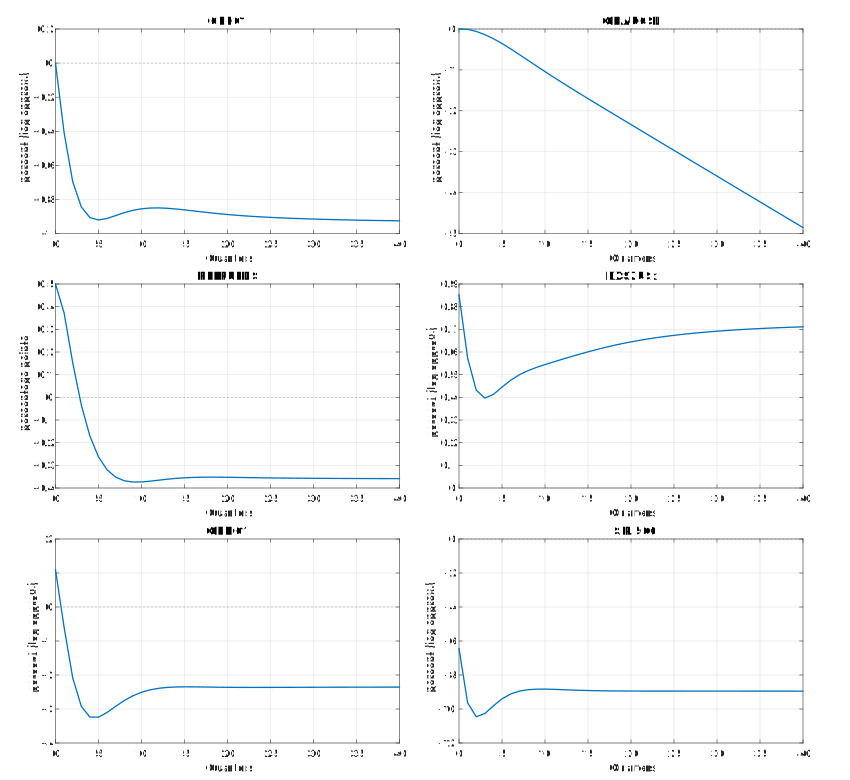
Notes: Seven static factors, four retained dynamic shocks, and one quarterly VAR lag are estimated from the 242-by-210 classroom panel. The monetary-policy impact is 0.5 percentage points. Logged series are cumulated according to their source transformation codes and multiplied by 100. The figure reports point estimates, not bootstrap confidence bands. The exchange-rate label refers to the supplied EXSZUSx series; the transformed MAT file does not permit an independent reconstruction of its raw-data definition.
6 The connection to filtering
A state-space model describes both state transitions and measurements:
a_t=Ta_{t-1}+\eta_t,\quad \operatorname{Var}(\eta_t)=Q, \qquad y_t=Za_t+\epsilon_t,\quad \operatorname{Var}(\epsilon_t)=H.
Here a_t is k\times1, T and Q are k\times k, Z is n\times k, and H is n\times n. This representation can accommodate missing measurements without deleting the underlying transition date. It is a representation plus a set of parameter assumptions, not by itself an alternative estimate of the empirical model above.
For predicted mean a_{t|t-1} and covariance P_{t|t-1}, the innovation is v_t=y_t-Za_{t|t-1} and its covariance is F_t=ZP_{t|t-1}Z'+H. The update is
K_t=P_{t|t-1}Z'F_t^{-1},\qquad a_{t|t}=a_{t|t-1}+K_tv_t.
The implementation solves covariance systems and uses the Joseph form
P_{t|t}=(I-K_tZ)P_{t|t-1}(I-K_tZ)'+K_tHK_t'
to reduce numerical loss of positive semidefiniteness. Cholesky factors also provide a stable observed-data log likelihood.
When only some series are observed, the update uses the corresponding rows of Z and submatrix of H. When all are missing, the prediction becomes the posterior and that date contributes zero measurement log likelihood. The next transition still occurs. Each row of the input must represent one regular transition interval: an unrecorded calendar gap must be inserted as missing rows, not compressed into a single step.
The supplied initial mean and covariance describe the first observation date, before its measurement update. This convention is stated explicitly because predicting once before the first update would imply a different prior. The scalar example in filterExample has known parameters and is checked against hand calculations. No empirical EM algorithm, parameter likelihood optimization, mixed-frequency observation equation, or real-time vintage evaluation is claimed here.
7 Reading the implementation
Read the data assertions in replicate.m, then the IC2 and rank-reduction steps in tsma.factor.dynamic. The shared recursive rotation can be read independently of factor estimation. tsma.factor.kalman belongs to the separate filtering extension, not to the two-step empirical fit.
% Declare the two-step structural DFM choices from the actual classroom MATLAB script.
function cfg = config()
% The transformed panel is a course MAT file without an embedded date vector.
cfg.inputName = fullfile('session10','factor_data.mat');
% Pin those exact transformed-panel bytes rather than an unverified later vintage.
cfg.inputSHA256 = 'ef34075acfa3d46fb6bc9a907b5bc027eb5b4a977f5f31cb9a60dd94a0c8eadc';
% Compare one through twenty static factors with the Bai-Ng IC2 criterion.
cfg.maximumFactors = 20;
% Four dynamic shocks approximate innovations in the larger static-factor VAR.
cfg.shocks = 4;
% Classroom BIC selects among one through four quarterly VAR lags.
cfg.maximumLag = 4;
% Report ten years after the monetary-policy innovation.
cfg.horizon = 40;
% Identify a recursive monetary-policy shock with the policy rate ordered third.
cfg.identifyingNames = ["GDPC1","CPIAUCSL","FEDFUNDS","EXSZUSx"];
% Return the data, static-factor, dynamic-shock, and identification choices.
end
The saved empirical object includes the complete transformed panel, normalization, factor criterion, VAR coefficients and residuals, innovation eigenvalues, retained-rank impact matrix, structural rotation, unit-variance shocks and reporting scale. The benchmark compares the classroom point responses in observed units; it does not equate arbitrarily signed factor coordinates or claim to reproduce the source’s bootstrap bands.
The source comparison on MATLAB R2024a gives a maximum difference of 2.665\times10^{-15} over the twenty IC2 values, 3.464\times10^{-14} in the common component, and 4.332\times10^{-11} across all 8,610 monetary-policy response entries. These comparisons use the same source data and policy normalization; they are not comparisons with the original paper’s published estimates.
8 Exercises
1. What rank reduction discards
Let \Sigma_F=\operatorname{diag}(9,4,1) and retain q=2 shocks. Construct R, calculate RR', the discarded covariance and the retained variance share. For an innovation \varepsilon=(3,2,5)', find the standardized retained shocks and reconstructed innovation.
Hint: The retained eigenvectors are the first two coordinate vectors.
2. Policy-shock units
A unit-variance structural shock raises the federal funds rate by 0.2 percentage points and moves GDP by -0.003 log points at horizon four. Rescale the response to a fifty-basis-point tightening. State the GDP response in approximate percent. Explain why multiplying every other structural shock by the same factor is unnecessary.
Hint: Fifty basis points equals 0.5 percentage points, not 50 points.
3. A missing observation
Consider a_t=0.8a_{t-1}+\eta_t, Q=0.36, and y_t=a_t+\epsilon_t, H=0.25. The first-date prior is N(0,1) and the observations are (1,\text{missing},0). Work out all three filtered means and variances. Calculate the first log-likelihood contribution.
Hint: A missing measurement skips the update, not the transition.
4. The factor penalty
For a panel with T=200, N=100, suppose V(1)=0.50, V(2)=0.46, and V(3)=0.43. Calculate IC2 at each candidate count and choose the minimum. How would the conclusion differ if only the unpenalized reconstruction error were considered?
Hint: The penalty per factor is (N+T)\log(\min(N,T))/(NT).