Factor-augmented VARs
Session 09 · Lecture notes
A monthly credit-shock application augments an observed spread with four principal components from a large macroeconomic panel. These notes explain the transformation and normalization rules, the measurement regression, and identification through restrictions on observed variables. A source-compatible calculation isolates the classroom script’s metadata-row convention.
1 A credit shock in a large panel
A small VAR uses only the variables that appear in its equations. If households, firms, and policymakers observe a much larger information set, the resulting residual may mix an unexpected disturbance with a response to omitted information. A factor-augmented VAR addresses this problem by summarizing a large panel in a small number of estimated factors. It also provides responses for variables outside the VAR itself (Bernanke et al. 2005).
The BSE financial-shock exercise follows the approach of Boivin et al. (2020), using a FRED-MD panel, four principal components, and an observed corporate credit spread. The exercise is not a replication of that paper’s complete mixed-frequency dataset: it uses new orders for durable goods rather than the paper’s investment measure. I retain the classroom application and separate two source-code conventions from the preferred implementation.
This chapter assumes the VAR and recursive identification material. The new issues are panel preparation, factor normalization, the distinction between factor loadings and measurement-regression coefficients, and the mapping from a small system back to observed macroeconomic variables.
2 Preparing the monthly panel
The workbook contains a row of transformation codes before the dated observations. That row is metadata. It must not be differenced against the first observed month. The preferred importer removes it before applying any transformation. Columns containing a missing observed level are excluded, matching the classroom balanced-panel policy; their names are retained in data.excludedNames. Missing values are never replaced by zero.
The constructed spread is BAA_t-GS10_t, in percentage points. It is added to the panel and later retained as an observed factor. FRED transformation codes are applied column by column:
| Code | Transformation | Initial unavailable rows |
|---|---|---|
| 1 | x_t | 0 |
| 2 | \Delta x_t | 1 |
| 3 | \Delta^2x_t | 2 |
| 4 | \log x_t | 0 |
| 5 | \Delta\log x_t | 1 |
| 6 | \Delta^2\log x_t | 2 |
| 7 | \Delta(x_t/x_{t-1}-1) | 2 |
The common sample begins after the two genuine initial differences. The preferred panel has 754 months, March 1959 through December 2021, and 106 series including the constructed spread. It includes the pandemic period. The source-compatible calculation instead begins in February 1959 because the source inadvertently counted the metadata row as an observation. The compatibility result is retained separately, not substituted into the preferred figure.
Dropping an entire incomplete column is simple and reproducible, but not innocuous. It favors series available throughout the full historical sample. It is not an imputation method and is not appropriate for a real-time ragged-edge nowcast. Nor should the full-sample column-selection rule be described as a real-time information set.
3 Principal components
Let X be the T\times N transformed panel. Standardize each column using its estimation-sample mean and sample standard deviation:
Z_{ti}=\frac{X_{ti}-\bar X_i}{s_i}.
For the singular-value decomposition Z=USV', retain the first r=4 columns V_r and define
F=ZV_r,\qquad \widehat\chi=FV_r',\qquad \widehat\xi=Z-\widehat\chi.
The loading columns have unit Euclidean length, V_r'V_r=I_r. The factors themselves do not have unit variance under this normalization: their variances equal the corresponding panel-covariance eigenvalues. Mixing this convention with F'F/T=I without changing the loadings would change the reconstructed panel.
Factor signs have no economic content. Multiplying a loading column and its factor by minus one leaves FV_r' unchanged. The implementation chooses signs deterministically by making each loading vector’s largest absolute entry positive. Benchmarks compare common components and identified observed-variable responses, not arbitrary raw factor signs.
For forecasting, means, standard deviations, and loadings must be estimated on the training sample alone. tsma.factor.pca accepts explicit training rows and then projects later observations onto those fixed loadings. A unit test changes only a future observation and verifies that no training quantity changes. The historical exercise here deliberately uses its full sample; its fitted factors are not real-time estimates.
4 The augmented state
Let s_t be the observed credit spread and form the five-dimensional state v_t=(s_t,F_t')'. Estimate
v_t=c+A_1v_{t-1}+\cdots+A_pv_{t-p}+u_t, \qquad E(u_tu_t')=\Sigma.
The classroom BIC convention selects two monthly lags. As in Session 08, the source criteria use changing lag samples and the initial input count in their covariance and penalty. The result object records that policy. The final VAR covariance, by contrast, uses its actual residual degrees of freedom.
The PCA loadings alone are not the complete measurement equation because the augmented state also includes the observed spread. Regress the unstandardized transformed panel on an intercept and all five states:
X_t=a+\Lambda v_t+\eta_t.
In code, measurementBeta has six rows and N columns. Its first row is the intercept; the transpose of the remaining rows is \Lambda. QR solves this regression without forming an explicit inverse. The saved idiosyncratic component permits the exact check X_t-a-\Lambda v_t-\eta_t=0.
The implied response is a response of the common component conditional on no direct response of \eta_t to the identified shock. Mapping back to an observed series does not eliminate that assumption.
5 Identifying the credit shock
First compute an arbitrary orthogonal factor-system impact matrix S=\operatorname{chol}(\Sigma) and responses \Lambda C_hS. These shock columns do not yet have the desired observable interpretation. Select five observed variables in the explicit order
(PCEPI, UNRATE, AMDMNOx, FEDFUNDS, BSPREAD).
Let B_0 be their five-by-five impact block. If it is nonsingular, set
L=\operatorname{chol}(B_0B_0'),\qquad H=B_0^{-1}L.
Here Cholesky means the lower triangular factor. Since LL'=B_0B_0', the implied rotation satisfies HH'=I. The identified panel responses are \Lambda C_hSH.
The fifth shock raises the credit spread while having zero impact on the first four identifying observables. Those zero responses are assumptions, not empirical evidence that prices, unemployment, orders, and the policy rate cannot move contemporaneously. The shock has unit variance under the estimated state innovation covariance; it is not normalized to a one-percentage-point change in the spread.
The source finds identifying rows by spreadsheet position, producing UNRATE, AMDMNOx, FEDFUNDS, PCEPI, BSPREAD. The preferred implementation uses the written name list instead. Both leave credit ordered last; the interpretation of the other shock columns differs. Every reported result stores its actual order.
6 Response units
Differencing must be undone along the horizon dimension, not across variables or shocks. For a first-differenced series, b_h^{level}=\sum_{j=0}^{h}b_j^{difference}. A second-differenced series requires two cumulative sums. Logged responses remain log changes; multiplication by 100 expresses the usual small-change percentage approximation. A rate already measured in percentage points must not be multiplied by 100.
Code 7 is different. Summing its response does not recover a level response without information about the baseline path and the nonlinear growth-ratio mapping. The exporter leaves those response units unchanged instead of claiming to undo a nonlinear transformation.
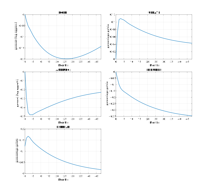
Notes: The figure uses the preferred 754-month panel, four principal components and the observed credit spread. The shock is the fifth column of the observable recursive identification. The first four identifying variables have zero impact responses. PCE prices and new orders are reported as 100 times cumulative log responses; the rates and spread are in percentage points. The lines are point estimates without sampling bands.
7 What the code saves
replicate.m stores the standardized panel, factors, loadings, excluded names, full VAR, both measurement and VAR residuals, all identified response columns, transformation codes, and source-compatible estimates. The following executable configuration fixes the baseline choices.
% Specify the monthly credit-shock FAVAR and its identifying order.
function cfg = config()
% Keep the classroom workbook in a session-specific ignored raw-data directory.
cfg.inputName = fullfile('session09','fred_md_final.xlsx');
% Pin the original workbook rather than silently downloading a revised FRED vintage.
cfg.inputSHA256 = '22dbd5ec1fdf81f7b2611dbcb98ab54378b221303fc3a3370ca0c48ef274e2b6';
% Four estimated factors supplement the observed BAA-minus-Treasury credit spread.
cfg.factors = 4;
% Choose the VAR lag by classroom BIC among one through five months.
cfg.maximumLag = 5;
% Four years of monthly responses retain impact as an additional array slot.
cfg.horizon = 48;
% Resolve the order by names rather than the source's spreadsheet-position search.
cfg.identifyingNames = ["PCEPI","UNRATE","AMDMNOx","FEDFUNDS","BSPREAD"];
% Return all data, factor, lag, horizon, and ordering choices.
end
Read tsma.factor.read_monthly before tsma.factor.favar. The former determines which observations and series exist; the latter estimates the model from that prepared panel. tsma.factor.recursive then implements the observable rotation as a separate testable operation.
The replication verifies the classroom point-estimate calculation. It does not reproduce the original bootstrap bands. A suitable uncertainty exercise must specify whether factors and loadings are re-estimated, how serial and cross-sectional dependence in idiosyncratic components is preserved, and whether the balanced-panel rule is held fixed. Applying a small-VAR residual bootstrap while treating estimated factors as observed would answer a narrower conditional-inference question.
The source-compatible benchmark has an exactly matching transformed panel. Its largest common-component difference is 6.395\times10^{-14} and its largest difference over all 25,970 integrated response entries is 1.597\times10^{-13}. The legacy workbook loader returns no text output on the tested MATLAB R2024a macOS installation, so the comparison supplies the same header and numeric rectangles with readcell and readmatrix, then runs the unchanged numerical source blocks. The saved report names that loader adjustment; it does not claim an unmodified legacy import.
Session 10 keeps the large-panel measurement equation but distinguishes the number of static factors from the number of underlying dynamic shocks.
8 Exercises
1. Normalization and reconstruction
For Z=\begin{pmatrix}-1&-1\\0&0\\1&1\end{pmatrix}, find the first loading vector, factor scores, covariance eigenvalue, common component, and idiosyncratic component. Show why the factor does not have unit sample variance under the stated normalization.
Hint: The two columns are identical and each has sample variance one.
2. An observable rotation
Let B_0=\begin{pmatrix}1&2\\3&1\end{pmatrix}. Compute L=\operatorname{chol}(B_0B_0'), solve B_0H=L, and verify that H'H=I. Which impact is restricted to zero by this order?
Hint: The lower Cholesky factor has first column (\sqrt5,\sqrt5)'.
3. Cumulating responses
A response to a second difference is (1,0,0) at horizons zero, one, and two. Calculate the response of the first difference and the level. Repeat for (0.01,-0.002,0) in the first difference of a log series, reporting approximate percentage changes.
Hint: All cumulative sums run over horizons, beginning with impact.
4. A metadata row
A workbook has 756 real monthly observations preceded by one row of transformation codes. The largest transformation is a second difference. Calculate the preferred common-sample size and the size obtained if the metadata row is mistakenly treated as data. Explain why deleting the first two transformed rows does not necessarily remove all contamination.
Hint: A second difference at the second real observation still uses the metadata value two rows earlier.