Quantile SVARs and growth risk
Session 08 · Lecture notes
The classroom application estimates conditional quantiles of quarterly GDP growth and identifies innovations in lower, total, and upper tail widths. I derive the check-loss optimization problem, verify its numerical solution with a primal-dual certificate, and connect the fitted quantiles to restricted VAR responses. The discussion distinguishes distribution innovations from exogenous structural shocks.
1 Growth risk
A forecast of average growth does not tell us how much probability lies in the lower tail. Two quarters can have the same median forecast and very different downside risks. This session asks how an innovation that widens the predicted growth distribution is associated with subsequent movements in output, unemployment, investment, and financial variables.
The application follows the quantile-SVAR exercise in the BSE materials, which draws on Downside and Upside Uncertainty Shocks (Forni et al. 2021) and the conditional-growth approach of Adrian et al. (2019). I reproduce the classroom specification, not the complete published-paper analysis. The quantile regression supplies a measure of distributional risk; a linear VAR supplies its dynamic propagation. These are separate estimation steps.
The prerequisites are linear regression, the VAR moving-average representation, and the distinction between a conditional expectation and a conditional quantile. By the end of the exercise, the relevant checks are concrete: the growth target must be dated correctly, the optimization must satisfy a numerical certificate, and the identified impact vector must have the stated variance and restrictions.
2 The quarterly sample
The private course CSV contains a FRED-QD vintage with two metadata rows. The replication selects variables by their recorded names. GDP and investment enter as 100 times their natural logs. Real equity prices are 100 times the log of the S&P 500 divided by the GDP deflator. Unemployment, the BAA-minus-ten-year yield spread, the ten-year-minus-three-month yield spread, and consumer sentiment remain in their source units.
Write the seven-variable predictor vector as
z_t=(\log GDP_t, U_t, \log I_t, \log SP_t^{real}, CS_t, TS_t, Sent_t)',
where the three logged series above are scaled by 100 in the code. The target is g_{t+1}=100(\log GDP_{t+1}-\log GDP_t): quarterly growth, not annualized growth. A coefficient of 0.2 therefore means 0.2 percentage points of quarter-on-quarter growth, not 0.2 percent of the GDP level.
| Object | First quarter | Last quarter | Rows |
|---|---|---|---|
| Predictor levels before lagging | 1960 Q1 | 2019 Q4 | 240 |
| Quantile-regression origins t | 1960 Q2 | 2019 Q4 | 239 |
| Growth targets t+1 | 1960 Q3 | 2020 Q1 | 239 |
The final target is in 2020 Q1 even though all predictor origins precede 2020. This is the source specification, not a strictly pre-pandemic target sample. A sensitivity exercise that drops that observation would be a changed specification and should be labelled accordingly.
3 Quantile regression
For each \tau\in\{0.1,0.5,0.9\}, estimate
\widehat\beta_\tau=\arg\min_b\sum_{t=1}^{T} \rho_\tau(g_{t+1}-x_t'b),\qquad \rho_\tau(u)=u\{\tau-\mathbf1(u<0)\}.
Here x_t contains an intercept, current GDP, unemployment, real equity prices and sentiment, followed by lagged unemployment and lagged real equity prices. It has seven columns. The loss weights a positive residual by \tau and a negative residual by 1-\tau. At the median the two weights are equal, so the objective becomes half the sum of absolute errors.
Unlike OLS, this objective is not differentiable at zero residuals. A solver that merely reports a small change in coefficients has not proved that it found the minimum. The implementation therefore also solves the dual problem
\max_a g'a\quad\text{subject to}\quad X'a=0, \quad \tau-1\leq a_t\leq\tau.
For any feasible a, g'a is a lower bound on the minimum check loss. The difference between the fitted primal loss and this dual value provides an observable optimality bound. The routine uses an interior logarithmic barrier, QR-scaled regressors, equality-constrained Newton steps, and backtracking that keeps every dual weight inside its box. It returns the weights, loss, feasibility error, and iteration count with the coefficients. The replication rejects a gap above 2\times10^{-5} or an equality error above 10^{-7}; it does not silently accept the iteration limit.
The three regressions are estimated independently. They need not produce ordered fitted quantiles at every date. crossingCount reports this diagnostic without rearranging predictions after estimation. This course sample has no crossings. That does not establish out-of-sample calibration: the fitted quantiles use the full estimation sample, and their regression form may be misspecified.
4 An innovation in tail width
Let z_t=c+A_1z_{t-1}+\cdots+A_pz_{t-p}+u_t, with E(u_tu_t')=\Sigma and moving-average matrices C_h, C_0=I. The course AIC calculation selects p=3 from one through eight lags. Its candidates have different starting dates and use the initial input count in the covariance and penalty. I retain that convention for the classroom comparison; it is not the common-sample criterion in Session 01.
Define the lower width as q_{0.5,t}-q_{0.1,t}, the total width as q_{0.9,t}-q_{0.1,t}, and the upper width as q_{0.9,t}-q_{0.5,t}. Let \gamma be the corresponding difference of current-quarter quantile coefficients, embedded into the seven-variable VAR order with zeros for unused predictors. Lagged predictors cannot contribute to the current surprise because they are already known at t-1. The width innovation is \gamma u_t and has variance v=\gamma\Sigma\gamma'. The unit-variance scalar shock and its response are
e_t=\frac{\gamma u_t}{\sqrt v},\qquad b_h=C_h\frac{\Sigma\gamma'}{\sqrt v}.
The covariance factor \Sigma is essential: \gamma' alone is a linear-combination direction, not a vector of variable impacts.
The lower, total, and upper width innovations are alternative shock definitions. They are generally correlated and are not three independent columns of a jointly identified structural system. Further, identifying an innovation in a fitted distribution does not by itself establish that it is an exogenous uncertainty shock. Other structural disturbances can move the same width.
5 Contemporaneous restrictions
The restricted exercise removes the component explained by the contemporaneous GDP, unemployment, and investment residuals. Let D select those three variables. The projected width direction is
\alpha=\gamma-\gamma\Sigma D'(D\Sigma D')^{-1}D.
The code implements the projection with a linear solve, not an explicit inverse. Then D\Sigma\alpha'=0, so
b_h^{R}=C_h\frac{\Sigma\alpha'}{\sqrt{\alpha\Sigma\alpha'}}
has zero impact on the three selected variables. Its later responses can be nonzero because C_h transmits the initial movement through lagged relationships. The restriction is substantive: it rules out within-quarter effects on these slow-moving variables. It does not prove that the remaining financial innovation is free of all confounding shocks.
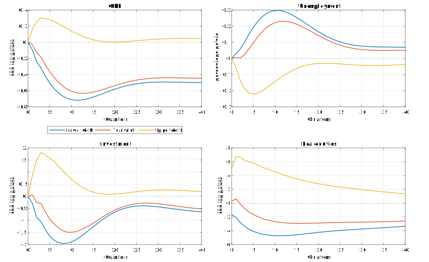
Notes: The three plotted paths correspond, in MATLAB’s line-color order, to lower, total, and upper width innovations. Each shock has unit variance under its own definition; the shocks are not mutually orthogonal. Horizons are quarters. Logged variables are measured in 100 log points and unemployment in percentage points. These are point estimates, not confidence intervals.
6 Reading the replication
Read config.m, then replicate.m, then tsma.quantile.fit. The entrypoint constructs one observed origin-target pair before repeating estimation across quantiles. It stores every VAR coefficient, residual, covariance, date, and quantile certificate in outputs/08-quantile-svars/replication.mat. The source below is included directly from the executable configuration.
% Declare the quarterly uncertainty-shock specification independently of the estimator.
function cfg = config()
% The original FRED-QD vintage is private input, not an automatically updated download.
cfg.inputName = fullfile('session08','quantilesvar_data.csv');
% Pin the exact classroom bytes before interpreting any numerical comparison.
cfg.inputSHA256 = '34a53f8500eea5d7c4dd9002f1bdb5ffd4aee80acdae922c680d7013627a4b40';
% Estimate lower-tail, median, and upper-tail conditional growth quantiles.
cfg.quantiles = [0.1,0.5,0.9];
% The source chooses its VAR lag by AIC among one through eight quarters.
cfg.maximumLag = 8;
% Report ten years of quarterly responses, with impact stored separately at slot one.
cfg.horizon = 40;
% Return the complete session specification.
end
The old source uses 240 observations in a covariance denominator after the VAR input has been shortened to 239. The preferred covariance uses the actual number of usable VAR rows minus regressors. The separate benchmark adjusts that scalar normalization before comparing response paths and records the change in revisions.md. Neither version supplies sampling uncertainty for the estimated quantile direction; inference would need to re-estimate both stages, not condition on the first-stage coefficients.
On MATLAB R2024a, the three primal-dual gaps are below 3.2\times10^{-7}. The optional comparison with the pinned original source gives the following maximum absolute differences after matching the covariance normalization:
| Compared object | Entries | Maximum difference |
|---|---|---|
| Quantile coefficients | 21 | 8.914\times10^{-7} |
| Fitted conditional quantiles | 717 | 2.398\times10^{-7} |
| Restricted response paths | 861 | 5.983\times10^{-7} |
These are numerical comparisons, not standard errors. The original solver has a looser optimization tolerance; the new solver also certifies its own objective bound independently of that comparison.
The next session changes the information set rather than the conditional moment. A FAVAR compresses a large macroeconomic panel into estimated factors while keeping the identifying restrictions visible.
7 Exercises
1. The forecast origin
A quarterly predictor sample runs from 1960 Q1 through 2019 Q4. The regression includes information at t and t-1 and predicts growth at t+1. Determine the first and last origins, targets, and sample size. Explain which GDP level is needed outside the predictor sample.
Hint: Count inclusive quarters after removing the first predictor row.
2. A quantile certificate
For y=(1,2,3,4,9)', fit an intercept-only median. Compute its objective. Construct feasible dual weights and show that their objective equals the primal objective. Why does this establish a global, rather than local, minimum?
Hint: At the median, nonzero residuals have dual weights \pm1/2.
3. A normalized distribution innovation
Let \Sigma=\begin{pmatrix}4&1\\1&1\end{pmatrix} and \gamma=(1,0). Calculate the unit-variance width shock’s impact vector. Then impose zero impact on the second variable. Compute the projected direction, its variance, and the restricted impact vector.
Hint: For the restriction use D=(0,1) before renormalizing.
4. The covariance denominator
The VAR has 239 input rows, seven variables, three lags and an intercept. Compute the unbiased residual covariance divisor. The source instead uses 240 as its initial row count. Derive how correcting that divisor changes a response normalized to a one-standard-deviation width innovation.
Hint: Multiplying \Sigma by c multiplies the normalized response by \sqrt c, not by c.