Nonlinear responses
Session 07 · Lecture notes
A response can depend on the state of the economy, the size of a shock, or both. These notes develop two distinct classroom applications: a smooth-transition fiscal VAR and a financial VAR-X with a squared-shock term. The discussion derives their estimators, checks numerical convergence, and distinguishes frozen-regime paths from generalized nonlinear impulse responses. Prerequisites: VAR estimation, structural identification, generalized least squares, and likelihood.
1 Two different nonlinearities
Does a spending shock have the same effect during a recession as during an expansion? Does doubling a financial shock double its effect? A linear, constant-parameter VAR answers yes to both by construction. Neither answer is an empirical finding of that model.
This session revisits two actual BSE applications. The first uses the supplied Auerbach-Gorodnichenko fiscal data and a smooth-transition model motivated by Auerbach and Gorodnichenko (2012). The second uses the classroom’s monthly financial panel and a quadratic-shock specification associated with Forni et al. (2022). I keep them separate: a state-dependent coefficient and a squared innovation represent different departures from linearity.
2 A smooth-transition fiscal VAR
Let x_t=(1,y_{t-1}',\ldots,y_{t-p}')' contain an intercept and lagged outcomes. With y_t ordered as log real government purchases, log real receipts, and log real GDP, write
y_t=(1-w_t)D_E'x_t+w_tD_R'x_t+u_t, \qquad \Sigma_t=(1-w_t)\Sigma_E+w_t\Sigma_R.
E labels the low-recession-weight regime and R the high-weight regime. The equation has a separate intercept and lag coefficients in each regime. The covariance also changes with the weight. The classroom weight is
w_t=F(s_{t-1})=\frac{1}{1+\exp(\gamma s_{t-1})},\qquad\gamma=1.5.
Low growth raises the recession weight. The sign of \gamma s in this formula matters: using 1/(1+\exp(-\gamma s)) would interchange the regime labels. At s=0, both weights equal one half. As \gamma grows, the transition approaches a threshold; with fixed positive \gamma, it remains smooth. These are not latent Markov-state probabilities.
The supplied fiscal data have 241 quarters, 1948Q4-2008Q4. Three lags leave 238 equation dates, 1949Q3-2008Q4. The source provides a seven-quarter growth-state series as Z0. I standardize that supplied series using its full-sample mean and sample standard deviation, matching the classroom, and use the preceding quarter’s standardized state for each equation.
This is retrospective conditioning. The MAT file does not by itself document a real-time vintage or establish that every ingredient of Z0 was observable at each historical forecast origin. A one-quarter lag alone cannot establish that stronger claim. Reconstructing the state from an explicitly backward-looking real-time panel would be a new specification, not an unnoticed data-cleaning change.
% Evaluate recession weights without overflow in either tail.
function weight = logistic(state, gamma)
% A positive slope makes low standardized growth correspond to high recession weight.
assert(isscalar(gamma) && isfinite(gamma) && gamma > 0 && all(isfinite(state(:))), 'tsma:Transition', 'Finite states and positive gamma are required.');
% Use tanh to avoid exp(+large), which can produce an undefined infinity ratio.
weight = 0.5 * (1 - tanh(0.5 * gamma * state));
% Return values in [0,1], including limiting tail values.
end
The hyperbolic-tangent expression equals the logistic formula algebraically but avoids the Inf/Inf problem of directly evaluating \exp(-\gamma s)/(1+\exp(-\gamma s)) in an extreme tail.
3 Conditional estimation
Because \gamma and the state sequence are fixed here, the conditional mean is linear in the regime coefficients. Its design row is X_t=((1-w_t)x_t',w_tx_t'). Initial OLS gives residuals from which to start estimating the covariance parameters.
For given coefficient estimates, minimize the Gaussian negative log likelihood
\mathcal L=\frac{Tn}{2}\log(2\pi)+ \frac12\sum_{t=1}^{T}\left\{\log|\Sigma_t| +u_t'\Sigma_t^{-1}u_t\right\}.
Each regime covariance is parameterized as LL'. The free parameters are the lower-triangular entries of L, with its diagonal stored in logarithms and exponentiated when the covariance is evaluated. This enforces a positive diagonal and avoids unconstrained proposals for covariance entries that would produce an indefinite matrix. The likelihood uses Cholesky log determinants and triangular solves, not explicit inverses. The covariance calculation follows the classroom treatment of Lütkepohl and Netšunajev (2017); the spending-shock identification used below remains recursive rather than being inferred solely from variance changes.
Given the covariances, estimate the conditional mean by GLS. For each date, factor \Sigma_t=L_tL_t' and premultiply the stacked outcome and design block by L_t^{-1}. A QR least-squares solve on these whitened blocks gives the updated coefficients. This is algebraically equivalent to the classroom’s large block-diagonal weighting matrix, but it does not construct or invert that matrix.
Alternate the covariance and coefficient steps until both the relative coefficient movement and the likelihood change are small, with a successful inner optimizer flag. The base-MATLAB fminsearch routine replaces the original Optimization Toolbox dependency. In the checked run, convergence occurs in seven outer iterations. The log likelihood, including its normalizing constant, is 2018.203067. The last relative coefficient change is 3.81\times10^{-6} and the last objective change is 7.88\times10^{-8}.
This is numerical convergence from the declared deterministic start, not a proof of a global likelihood maximum. The saved trace makes that claim auditable. The returned GLS covariance conditions on the state sequence and estimated covariance matrices. It is not the full joint parameter covariance and does not supply confidence bands for nonlinear responses.
4 Frozen regimes are not evolving states
To reproduce the classroom comparison, extract each regime’s lag matrices and compute its ordinary Wold recursion while holding the regime fixed. Identify a spending shock recursively with purchases first. Normalize its impact on log purchases to 0.01 and multiply the plotted log responses by 100. The resulting purchase impact is one percent in each regime.
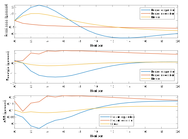
The shock raises real purchases approximately one percent on impact. Every outcome is plotted in approximate percent units. Expansion and recession paths keep their respective regime coefficients and covariances fixed at every horizon. They are not generalized impulse responses with an endogenous future state, and no bootstrap confidence band is shown.
In these frozen-regime calculations, GDP rises about 0.0732 percent on impact in expansion and 0.1700 percent in recession. These are log-response comparisons, not dollar multipliers. A dollar multiplier additionally requires an output-to-spending level conversion and a definition of whether responses are impact, peak, or cumulative. Applying one full-sample ratio to both regimes can change the economic comparison; Session 06 develops a cumulative-IV alternative with explicit units.
A generalized nonlinear response instead compares two conditional paths from the same initial history and integrates over the same future innovations. If the state is determined by past output, the initial shock can change later weights and therefore later coefficients. Keeping those weights fixed answers a different counterfactual. The distinction goes back to Koop et al. (1996). The repository does not present a frozen-regime path as an estimated generalized response or attach a new state-transition law to the source’s supplied state series without justification.
Companion roots for each frozen regime are retained as diagnostics. Their largest moduli are approximately 0.9957 in expansion and 1.0024 in recession. The recession-limit VAR is therefore slightly explosive. I report finite-horizon responses, not stationary long-run multipliers for that regime. Stability of each isolated regime would not, by itself, prove global stability of a nonlinear switching process. Finite-horizon response calculations and asymptotic stability claims must be kept separate.
5 A quadratic financial shock
The second application uses monthly data from January 1973 through August 2016. The source panel combines FRED macroeconomic series, an excess bond premium, stock prices, and a shadow short rate. The revised importer matches their actual monthly identifiers and explicitly applies the classroom shadow-rate splice beginning in August 2008. No missing value is converted to a zero.
After differencing log CPI once, the vector contains 100\log IP, 100\Delta\log CPI, unemployment, EBP, the financial conditions index, 100\log real stock prices, and the short rate. A five-lag recursive VAR has 518 residual months. The fourth Cholesky shock is the EBP innovation; positive values mean a tightening under this orientation. I retain the classroom’s sample-standard-deviation scaling of that recovered shock.
The nonlinear conditional mean is
y_t=c+\sum_{\ell=1}^{p}A_\ell y_{t-\ell} +a\eta_t+b\eta_t^2+v_t.
The first three equations exclude both contemporaneous shock terms. The EBP equation includes the linear term but excludes the square. The final three equations include both. These are identifying restrictions, not automatic properties of OLS. They let the linear EBP innovation be recovered while allowing contemporaneous asymmetry in faster-moving variables.
Each equation is estimated with its permitted columns; excluded coefficients are stored as exact zeros. The full fitted objects retain coefficients, residuals, dates, and HC0 covariances conditional on the generated shock regressor. Those covariances ignore first-step shock-estimation uncertainty and do not justify a structural-response confidence band by themselves.
Let C_h be the Wold matrices of this fitted VAR-X. The response comparing a shock of size \delta with a zero shock, holding other innovations fixed, is
r_h(\delta)=C_h(a\delta+b\delta^2).
Therefore r_h(2)=2C_ha+4C_hb, not 2r_h(1). A negative shock reverses the linear part but leaves the squared part unchanged. Responses are relative to \eta=0, not relative to the unconditional mean of \eta^2, which is nonzero. This distinction matters for interpreting the baseline and intercept.
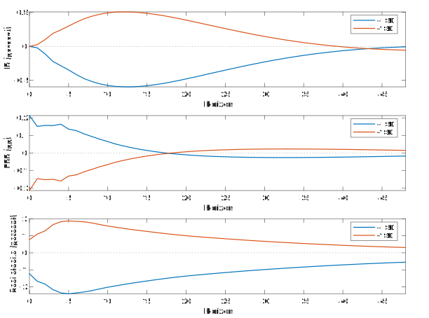
Positive shocks raise the excess bond premium under the classroom ordering. The +1 SD and -1 SD impacts on EBP are approximately +0.2134 and -0.2134 percentage points. Real-stock impacts are approximately -1.2337 and +0.7762 percent, illustrating the squared term’s asymmetry. These are classroom point estimates, not a new replication of every result in Forni and coauthors.
6 What the audit establishes
verify_session07 compares the revised GLS update with the original routine at identical covariance matrices and states. It also checks the original likelihood after accounting for its omitted Gaussian constant. The financial VAR-X coefficients are compared with an independent implementation of the classroom normal equations, equation by equation. An additional verify_financial07 audit re-estimates the original VAR, recovers and standardizes its financial shock, refits the constrained VAR-X, and uses the original companion-power recursion to compare all 1,372 response entries across seven outcomes, 49 horizons, and four shock sizes.
These checks separate the mathematical refactor from an optimizer-path claim. The revised program does not claim that fminsearch follows the original fminunc trajectory or reproduces an unverified saved bootstrap. The original bootout.mat is not loaded. Both empirical applications run on fingerprinted source inputs; the raw files and original helpers remain outside the public distribution.
7 Exercises
State weights and timing
For F(s)=1/(1+e^{1.5s}), calculate F(-1), F(0), and F(1). In a VAR with observations t=1,\ldots,8 and three lags, which state observations belong to the five fitted equations? Why is full-sample standardization not a real-time forecasting procedure?
Hint: The equation at t uses F(s_{t-1}).
Whitening a likelihood
In a scalar model, residuals are (2,3)' and conditional variances are 4 and 9. Calculate the negative Gaussian log likelihood, including its constant. What changes if the constant is omitted? Explain why equal regime covariances reduce GLS coefficients to OLS when every equation has the same regressors.
Hint: Divide each residual by its conditional standard deviation.
A state that changes after impact
Consider y_t=a(s_{t-1})y_{t-1}+\varepsilon_t, where a=0.8 for s<0 and a=0.2 otherwise. Set s_t=y_t, y_{t-1}=-1, and compare a unit shock with a zero shock, with subsequent innovations zero. Find the impact and horizon-one differences. Compare the latter with a response that freezes the initial regime forever.
Hint: Determine the next regime separately on the shocked and unshocked paths.
Shock size and asymmetry
At a given horizon, suppose C_ha=-0.5 and C_hb=-0.2. Calculate responses to shocks +1,-1,+2,-2. Recover the linear and quadratic components from the responses to +1 and -1. What is the baseline being compared with each shock?
Hint: Add and subtract the positive and negative unit-shock responses.