Local projections and fiscal multipliers
Session 06 · Lecture notes
These notes examine the response of output and government purchases to military-spending news using Ramey and Zubairy’s quarterly data. Local projections estimate the responses at each horizon. A cumulative instrumental-variables regression then relates the output response to the induced change in purchases. The discussion covers HAC inference and state dependence, with an annotated MATLAB replication of the BSE classroom specification. Prerequisites: ordinary least squares, instrumental variables, and basic matrix algebra.
1 Fiscal news
A spending announcement and a spending increase are not the same event. An announcement can change expectations today even if the purchases arrive over several years. We first estimate how output and government purchases respond to military-spending news. We then ask how much cumulative output changes per dollar of cumulative purchases associated with that news.
The distinction matters for both the regression and its interpretation. A coefficient on news is a response to the news measure. It becomes a spending multiplier only after relating that response to the induced change in purchases. A narrow confidence interval does not establish that the news is a valid instrument.
The application follows the BSE local-projections exercise associated with Ramey and Zubairy (2018). The course code is the numerical reference; the published paper is the source of the data and empirical design. This session does not replicate every specification or published table. In particular, the course uses a fixed horizon-dependent HAC rule, whereas the authors’ Stata package also implements different bandwidth and weak-instrument procedures.
We begin with the normalization of the data and the timing of each regression. The linear model provides the basis for cumulative IV multipliers and, subsequently, for responses that depend on the initial unemployment rate. The MATLAB implementation follows the same order.
2 The data
Normalization
The input is RZDAT.xlsx, sheet rzdat. The importer checks its SHA-256 fingerprint, required column names, positive observed denominators, and quarterly index before estimation. The workbook has 564 rows; the configured 1889 Q4-2015 Q4 window contains 505 quarters. The regression sample is smaller because observations also need complete lags and a future outcome at the chosen horizon.
Write Y_t for real GDP, G_t^N for nominal government purchases, P_t for the GDP deflator, and Y_t^* for the supplied sixth-order-trend potential GDP series. The regressions use
y_t=\frac{Y_t}{Y_t^*},\qquad g_t=\frac{G_t^N/P_t}{Y_t^*},\qquad z_t=\frac{N_t}{P_{t-1}Y_{t-1}^*}, \tag{1}
where N_t is the military-spending news series. Output and purchases are ratios to current potential GDP; news is a ratio to last quarter’s nominal potential GDP. These variables are not logarithms or growth rates. The potential-output estimates and narrative news are supplied inputs, not series reconstructed in this repository.
A news innovation of 0.01 is one percentage point of lagged nominal potential GDP. If its LP coefficient is b_h, the induced change in the outcome ratio is 0.01b_h. Multiplying that response by 100 expresses it in percentage points of potential GDP. Those are the units shown in the response figure.
Initial news
News is missing in 1889 Q4. The classroom loop begins assigning normalized news at the second observation; MATLAB fills the earlier, unassigned element with zero. The zero arises from array allocation; it does not represent an observed value of the news series.
The main run preserves the missing value. With four lags of news, the first complete origin is 1891 Q1, giving 500 observations at impact. The classroom-zero option is used only in the compatibility audit. It reproduces the old convention and admits 1890 Q4, giving 501 impact observations. Both runs use the same unmodified workbook.
Calendar alignment
The workbook represents a quarter as a decimal year. For example, 1890.75 means 1890 Q4. Multiplying by four gives an integer index: the next quarter’s index is exactly one larger. We validate this property rather than rounding unrecognized dates into apparently valid ones.
At horizon four, an origin of 1891 Q1 must be paired with the outcome in 1892 Q1. Its controls include 1890 Q1 through 1890 Q4, not four arbitrarily adjacent rows. If an intermediate date is absent, a cumulative outcome is missing even when its endpoint is observed.
| Origin t | Response y_{t+4} | Latest control | Earliest control | State information |
|---|---|---|---|---|
| 1891 Q1 | 1892 Q1 | 1890 Q4 | 1890 Q1 | Unemployment in 1890 Q4 |
| 1891 Q2 | 1892 Q2 | 1891 Q1 | 1890 Q2 | Unemployment in 1891 Q1 |
The lookup used throughout the replication is short enough to read in full. values is T\times m; periods is T\times1; offset is an integer. available identifies genuine matches, and location tells MATLAB which input row contains each requested date. No observation is moved across a gap.
% Return values at quarter t + offset; absent calendar quarters stay missing.
function shifted = calendar_shift(values, periods, offset)
% Require one row of data per integer quarter; columns may be multiple series.
assert(size(values, 1) == numel(periods), 'tsma:Dimensions', 'Rows must match dates.');
% Standardize dates as a column so array expansion cannot alter lookup.
periods = periods(:);
% Reject duplicate, unordered, or fractional quarter identifiers.
assert(all(isfinite(periods)) && all(periods == fix(periods)) && all(diff(periods) > 0), 'tsma:Dates', 'Dates must be unique increasing integer quarters.');
% A positive integer requests a lead; a negative integer requests a lag.
assert(isscalar(offset) && isfinite(offset) && offset == fix(offset), 'tsma:Offset', 'Offset must be an integer.');
% Allocate the original shape with missing values for unavailable dates.
shifted = NaN(size(values));
% Match requested dates to observed dates instead of shifting adjacent rows.
[available, location] = ismember(periods + offset, periods);
% Copy only genuine matches, retaining every series in the matched row.
shifted(available, :) = values(location(available), :);
% End the calendar lookup function.
end
3 Local projections
Local projections estimate a separate regression for each horizon rather than iterating a fitted dynamic system forward (Jordà 2005). For outcome v\in\{y,g\}, the linear specification is
v_{t+h}=a_h+b_h^v z_t+ \sum_{j=1}^{4}\gamma_{h,j}' \begin{pmatrix}z_{t-j}\\y_{t-j}\\g_{t-j}\end{pmatrix} +u^v_{t+h}. \tag{2}
At h=0, the left-hand side is the contemporaneous outcome. At h=4, it is the outcome four quarters ahead, not the sum of the first five outcomes. Every coefficient, including the intercept and lag coefficients, is re-estimated at each horizon.
The design matrix
The linear design contains 14 columns: one intercept, current news, and twelve lagged controls. The controls are ordered by lag first, then variable: L1_news, L1_output, L1_spending, followed by the three second lags, and so on. The result object stores these names beside the numeric matrix. Plots locate news by its name rather than by an unexplained column number.
For a particular outcome and horizon, keep a row only if the future outcome and every required regressor are finite. The estimation calendar records origin dates t, not the dates t+h on the left-hand side. At horizon 20, the final origin is 2010 Q4, whose response is observed in 2015 Q4; the sample contains 480 observations.
Estimation
For one horizon, let X be the n_h\times14 complete-case design and let v_h collect its matched outcomes. OLS minimizes the sum of squared residuals. With X=QR, where Q'Q=I and R is upper triangular,
\widehat\theta_h=R^{-1}Q'v_h, \qquad \widehat u_h=v_h-X\widehat\theta_h. \tag{3}
The code evaluates the first expression with a triangular linear solve, R \ (Q' * y). It does not explicitly compute R^{-1} or invert X'X. Rank checks occur before estimation. If the design is singular, the coefficients are not uniquely determined and the function stops with an error identifying the failed check.
The coefficient b_h^v is a conditional regression response. A causal interpretation additionally requires the news innovation to be appropriately exogenous given the information set, with a correctly specified conditional response. Including four lags does not prove that requirement. War-related news may be associated with other events that affect output.
4 HAC inference
Horizon-h regression errors can be serially correlated, particularly when future response windows overlap. Heteroskedasticity can also change the variance over this long historical sample. We use a Bartlett HAC covariance following the convention in the classroom exercise (Newey and West 1987).
For score s_t=x_t\widehat u_t, define
\widehat S=\sum_t s_ts_t' +\sum_{\ell=1}^{L}\left(1-\frac{\ell}{L+1}\right) \sum_{t:\,t-\ell\text{ observed}} (s_ts_{t-\ell}'+s_{t-\ell}s_t'). \tag{4}
The inner sum uses dates exactly \ell quarters apart. Dropping a missing observation must not turn a two-quarter interval into a one-quarter interval. With unscaled sums as written here, the OLS covariance is
\widehat V_{OLS}=(X'X)^{-1}\widehat S(X'X)^{-1}. \tag{5}
There is no additional division by n_h and no n_h/(n_h-k) correction. The default maximum included lag is L=h+1: impact uses lag one, and horizon 20 uses lag 21. This preserves the classroom convention; it is not a claim that this rule is optimal for every application. The rule and actual lag are recorded in the exported tables.
The following function returns the regression estimates together with their covariance and estimation sample. The helper covariance.m applies the sandwich through triangular solves; hac_meat.m implements the dated score sums in Equation 4.
% Estimate y = X beta + u by QR and report Bartlett HAC inference.
function fit = ols_hac(y, X, bandwidth, periods)
% A single outcome column must align with the design and observation dates.
assert(iscolumn(y) && numel(y) == size(X, 1) && all(isfinite(y)), 'tsma:Dimensions', 'Outcome must be a finite n-by-1 vector.');
% Check rank and obtain the compact QR factors of the n-by-k design.
[Q, R] = tsma.inference.full_rank(X);
% Solve R beta = Q'y: ordinary least squares without normal equations.
fit.beta = R \ (Q' * y);
% Structural and fitted-regression residuals coincide for ordinary least squares.
fit.residual = y - X * fit.beta;
% Each row is x_t times u_t, the k-dimensional estimating-equation score.
scores = X .* fit.residual;
% Store the entire covariance matrix for tests and joint restrictions.
fit.covariance = tsma.inference.covariance(R, scores, bandwidth, periods);
% Clip only numerical roundoff below zero before taking standard-error roots.
fit.se = sqrt(max(diag(fit.covariance), 0));
% Record the retained sample size, not the pre-filtering data length.
fit.n = numel(y);
% Preserve exact origin dates for auditing each horizon's sample.
fit.periods = periods(:);
% Save the maximum included autocovariance lag in quarters.
fit.bandwidth = bandwidth;
% Return estimates, inference, residuals, and sample metadata together.
end
The plotted interval is \widehat b_h\pm1.96\,\mathrm{se}(\widehat b_h). It is a pointwise normal interval: coverage refers to a given horizon, not to the entire impulse-response path simultaneously. The method is asymptotic, and long horizons can be imprecise even when the initial dataset is large.
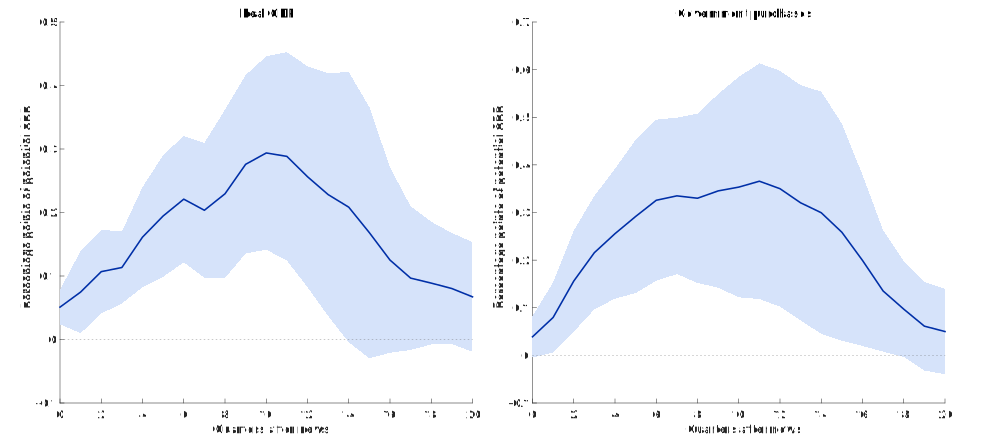
Notes: Outcomes are measured in percentage points of potential GDP. The shock is 0.01 in the normalized news series. The preferred sample retains missing initial news, uses four lags, and applies L=h+1 without a finite-sample multiplier. The figure is generated by the MATLAB replication.
5 Cumulative multipliers
Accumulated responses
A common descriptive calculation divides accumulated output responses by accumulated spending responses:
\widehat M_h^{ratio}= \frac{\sum_{j=0}^{h}\widehat b_j^y} {\sum_{j=0}^{h}\widehat b_j^g}. \tag{6}
This is not the response coefficient at horizon h. Nor can we obtain its standard error by dividing the individual standard errors: the numerator and denominator are estimated jointly and depend on many cross-horizon covariances. A denominator near zero also makes a ratio unstable. This replication therefore reports the ratio as a point estimate without a confidence interval.
Instrumental variables
Construct Y_{t,h}=\sum_{j=0}^{h}y_{t+j} and G_{t,h}=\sum_{j=0}^{h}g_{t+j}. At each horizon estimate
Y_{t,h}=M_hG_{t,h}+W_t'\delta_h+e_{t,h}, \qquad G_{t,h}\text{ instrumented by }z_t, \tag{7}
where W_t contains the intercept and four lags of news, output, and purchases. Current news is the excluded instrument; the included controls also appear in the instrument matrix. We do not sum the news instrument over future quarters. Today’s news is being used to explain the cumulative spending path associated with today’s information.
Relevance requires news to predict cumulative purchases after conditioning on W_t. Exclusion requires it to be uncorrelated with the structural disturbance in Equation 7. That is a substantive identifying assumption, not a property established by a first-stage statistic. The normalization follows the source exercise’s multiplier interpretation; it does not reconstruct counterfactual potential GDP under a spending intervention.
Let X=[G_h,W] and Z=[z,W]. With P_Z=Z(Z'Z)^{-1}Z', 2SLS uses \widehat X=P_ZX and
\widehat\theta_{IV}=(X'P_ZX)^{-1}X'P_ZY_h, \qquad \widehat e=Y_h-X\widehat\theta_{IV}. \tag{8}
The implementation forms the projection from a thin QR factorization of Z, then solves the second-stage regression by QR. Both rank conditions are checked. All stages use the same complete-case sample.
The IV covariance
Regressing Y_h on \widehat X gives the 2SLS point estimate, but the residual from that regression is not the residual of the structural equation. The IV covariance requires Y_h-X\widehat\theta_{IV}, evaluated at the actual endogenous regressor, not Y_h-\widehat X\widehat\theta_{IV}.
For the 2SLS sandwich, replace the OLS score in Equation 4 with \widehat x_t\widehat e_t and use bread (\widehat X'\widehat X)^{-1} on both sides. The code stores the complete matrix. A unit test checks it against the independently written, instrument-space moment formula in an overidentified example.
The classroom second-stage nwest call uses fitted-regression residuals. The compatibility audit reproduces those errors under the label classroomSE; the main tables and plotted IV interval use structural residuals. This distinction changes uncertainty without changing the 2SLS coefficient on a fixed sample.
Estimates and instrument relevance
At horizon four, the preferred cumulative-IV estimate is about 0.680, with a structural HAC standard error of 0.098. At impact it is about 1.306, with a standard error of 0.566. These are estimates from this specification, not a general statement that spending always has the same multiplier.
The impact first-stage HAC Wald statistic per excluded restriction is about 3.11. This raises a concern about relying on conventional normal inference. The statistic reported here is not a Kleibergen-Paap statistic, and there is no automatic “greater than ten” pass/fail rule. Partial R^2 and the full horizon-specific diagnostics are exported in multipliers.csv. This replication does not implement weak-instrument-robust intervals.
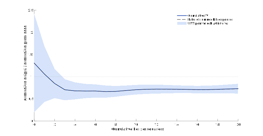
Notes: The shaded interval uses structural-residual HAC standard errors and is not weak-IV robust. The ratio sums coefficients estimated on different horizon-specific samples. Cumulative IV uses one common sample within each horizon. The two calculations need not be identical; their proximity here is an empirical result, not an imposed constraint.
6 State dependence
Define I_{t-1}=1\{U_{t-1}\geq6.5\}, with unemployment in percent. The state-dependent LP is
v_{t+h}=I_{t-1}X_t'\theta_h^H +(1-I_{t-1})X_t'\theta_h^L+u_{t+h}. \tag{9}
Here X_t includes the intercept, current news, and all lag controls. Every coefficient is allowed to differ, so the design has 28 columns. There is no additional unrestricted intercept: it would be collinear with the two state intercepts, since I_{t-1}+(1-I_{t-1})=1.
“High unemployment” describes the state just before the shock. It does not mean that unemployment stays above 6.5 percent for the entire response horizon. A state-dependent LP is not a simulated path that holds a regime fixed. Using contemporaneous unemployment instead would risk making the shock partly determine its own state classification.
The cumulative state-IV specification uses I_{t-1}G_{t,h} and (1-I_{t-1})G_{t,h} as endogenous regressors, with corresponding interactions of news as excluded instruments. Included controls are interacted too. The full instrument matrix enters the joint projection, and both state coefficients and their covariance are retained. The state results are available in the coefficient CSV and saved MATLAB object; a separate state-by-state first-stage and weak-IV analysis remains necessary before making strong comparisons of multipliers across regimes.
The old state-IV code drops one extra initial row before constructing lags. The compatibility audit preserves that restriction. The main implementation lets the explicit data-availability rule determine the sample. In this workbook, preserving missing initial news already excludes that origin.
7 MATLAB implementation
Entry points
From the repository root in MATLAB, result = run_session(6) runs the replication. run_tests() executes the unit and integration suites. Each result includes the configuration, exact input fingerprint, MATLAB version, coefficient vectors, full covariance matrices, and retained origin dates. Generated tables, vector figures, and the MATLAB object go to outputs/06-local-projections/.
The source-reading order follows the computation:
| File | What to understand before moving on |
|---|---|
config.m |
Dates, lags, horizons, threshold, units, and missing-news policy |
read_rz.m |
Named fields, normalization, calendar checks, and the input fingerprint |
design.m |
The order and information content of every regressor |
estimate.m |
One horizon, one sample mask, and one fit at a time |
ols_hac.m and hac_meat.m |
QR coefficients and dated score cross-products |
iv_hac.m |
Projection, structural residuals, and the IV sandwich |
export_results.m |
Unit conversions, labels, pointwise intervals, and sample metadata |
Every executable MATLAB line has an adjacent comment. Function signatures state what is returned; dimensions and units are introduced with the objects; loop comments distinguish the array position index from the economic horizon horizon. onCleanup restores temporary paths and closes only the file handles or figures opened by the current function. It does not clear the user’s workspace or suppress unrelated warnings.
Numerical checks
The test suite checks hand-calculated OLS and HAC examples, calendar gaps, missing cumulative outcomes, invalid dates, rank failures, changes of units, an independently derived IV covariance, and exact empirical sample endpoints. The IV-equals-OLS special case supplies another useful check: if the instruments equal the regressors, both coefficients and covariance must agree.
The optional verify_classroom(sourceDir) audit runs unchanged numerical blocks from the hash-verified classroom script using its original nwest.m and lagmakerMatrix.m. It excludes plots and editor-dependent setup, leaves all source files unchanged, and restores the working directory. All 2,646 compared coefficients and their 2,646 standard errors agree within 10^{-8}+10^{-7}|\text{reference}|. The largest absolute coefficient difference is about 1.55\times10^{-9}; the largest standard-error difference is about 1.45\times10^{-9}. This check includes controls, both outcomes, both state blocks, and all 21 horizons.
That agreement applies to the explicitly labeled classroom conventions. The preferred output preserves missing initial news and corrects IV inference. The source register records those changes separately. Agreement with a teaching script does not by itself validate identification, settle the bandwidth choice, or reproduce the published paper’s entire empirical exercise.
8 Exercises
1. Quarterly samples
The first usable origin is 1891 Q1 and the final outcome is 2015 Q4. Find the final origin and sample size at horizons zero, four, and twenty. Show the inclusive quarter-counting formula. Then suppose the outcome in 1950 Q2 is missing. List the origins that lose a horizon-four level outcome and those that lose a horizon-four cumulative outcome, considering outcome availability alone. Explain why using the next available row would give the wrong answer.
Hint: a level needs one endpoint; a cumulative outcome needs all h+1 dates from t through t+h. Express the affected cumulative origins as an inequality before listing their dates.
2. OLS and the HAC covariance
Let X=[\mathbf{1},(-3,-1,1,3)'] and y=(1.5,0.5,1.5,4.5)'. Calculate the OLS coefficients, residuals, and HC0 covariance. Verify the residual orthogonality conditions and report both standard errors. Separately, for scalar scores (1,2,3) on consecutive quarters, calculate the HAC meat with maximum lag one. Recalculate it when the scores occur at quarters 1, 3, and 4 instead.
Hint: the regressor is centered. HC0 uses unadjusted squared residuals; the lag-one Bartlett weight is one half. A HAC meat is only the middle of the sandwich, not yet a coefficient variance.
3. Structural residuals in IV
Why does running OLS on first-stage fitted regressors give the 2SLS point estimate but not automatically the right structural standard error? Derive the equality of the point estimates and write the two covariance formulas. Identify the line in iv_hac.m that makes the distinction. Does correcting the residual necessarily increase the standard error? Finally, show what happens when Z=X.
Hint: use the symmetry and idempotence of P_Z. Write the difference between the two residuals before comparing their score covariances.
4. A cumulative multiplier
At horizon four the preferred IV estimate is approximately 0.680 and its structural HAC standard error is 0.098. Calculate the displayed 95 percent interval. Are zero and one inside it? Interpret the coefficient’s units and the window represented by horizon four. Explain why the first-stage statistic is relevant even though it does not appear in that interval formula, and why a pointwise interval cannot be read as a confidence band for the entire response path.
Hint: distinguish sampling uncertainty conditional on the identifying assumptions from evidence for those assumptions. A cumulative horizon of four contains the impact quarter and four subsequent quarters.
5. Initial unemployment and state contrasts
Why does the state LP include two intercepts but no additional constant? What interpretation changes if the state uses unemployment in t rather than t-1? Derive a pointwise test of equal news coefficients using the full covariance matrix. Explain why the cross-state covariance need not vanish with HAC inference, even though each origin belongs to only one state.
For a numerical illustration, suppose the high- and low-state estimates are 0.8 and 0.4, both have variance 0.09, and their covariance is 0.08. Calculate the two individual 95 percent intervals and the interval for their difference. These numbers are a teaching example, not estimates from the fiscal dataset. What does the example show about comparing interval overlap?
Hint: write the difference as a linear contrast c'\widehat\theta. Its variance is c'\widehat Vc, including the off-diagonal terms.