External instruments
Session 05 · Lecture notes
An external instrument identifies the direction of a structural shock through its covariance with VAR innovations. These notes derive that moment ratio, establish the required monthly alignment, and reproduce the classroom monetary-policy application with the Gertler-Karadi and Miranda-Agrippino-Ricco instruments. They distinguish normalization from identification and first-stage diagnostics from weak-instrument-robust inference. Prerequisites: Sessions 01-03 and instrumental variables.
1 A proxy for the policy surprise
A policy announcement contains information that markets had anticipated and information they had not. A narrow-window asset-price movement can help measure the second component. It does not automatically equal a structural monetary-policy shock. The proxy-SVAR approach uses such a measure as an instrument for the shock rather than treating the measure as the shock itself.
The classroom application follows the approach of Gertler and Karadi (2015): estimate a monthly VAR containing real activity, prices, a policy indicator, and credit conditions, then identify a policy-impact direction using an external surprise series. The revised code uses the source’s actual input vintages and specification. It is a replication of this classroom exercise, not of all results in that paper.
2 The identifying moments
Let u_t=B\varepsilon_t, with orthogonal unit-variance structural shocks. The scalar instrument z_t targets shock j. Assume
E(z_t\varepsilon_{j,t})=\kappa\ne0,\qquad E(z_t\varepsilon_{k,t})=0\quad\text{for }k\ne j.
The first condition is relevance. The second excludes all other contemporaneous structural shocks. Then
m=E(u_tz_t)=b_j\kappa.
The observable covariance vector identifies the direction of b_j, but not its scale: both b_j and the instrument’s loading \kappa are unknown. Choose a policy indicator p for which m_p\ne0. Normalizing its impact to one gives
s=\frac{m}{m_p},\qquad s_p=1, \qquad \operatorname{IRF}(h)=C_hs.
This is a one-percentage-point innovation to the policy indicator if that indicator is measured in percentage points. It is not a one-standard- deviation innovation unless a separate variance normalization is applied. An alternative instrument unit, such as basis points rather than percentage points, multiplies both numerator and denominator and cancels.
One instrument identifies one direction. It does not identify the names or impact columns of the remaining shocks. A recursive ordering of the four variables is not used to identify this policy direction. The VAR’s ordering still matters for matching named series to their entries in the estimated vector.
3 Equivalence to the two-stage calculation
For simplicity, first consider the classroom’s no-intercept calculation over the instrument overlap. Regress the policy innovation on z: \widehat u_p=z(z'z)^{-1}z'u_p. Regress another innovation u_q on \widehat u_p. Its slope is
\frac{\widehat u_p'u_q}{\widehat u_p'\widehat u_p} =\frac{z'u_q}{z'u_p}.
Thus the second-stage slope equals the corresponding sample covariance ratio. With an intercept, first remove the overlap-sample means from both z and every innovation column, then use the same formula. Demeaning innovations over their full VAR sample is not the same operation: the instrument overlap is shorter and may have a different mean.
The source comments mention a constant, but the executable call is myols(...,0), which excludes it. I retain that calculation as result.classroom and use centered moments in result.proxy. The two versions therefore remain distinguishable. The comparison is a specification revision, not merely a faster way to calculate identical numbers.
4 Dates and units
The macro workbook covers January 1973-December 2009. Its transformed vector is
y_t=(100\log IP_t,\;100\log CPI_t,\;SR_t,\;EBP_t)'.
SR is the source’s short-rate/shadow-rate series, not a newly downloaded vintage. EBP is the excess bond premium. The first two responses are approximately percent changes; the last two are percentage-point changes. The twelve-lag VAR has 432 residual observations, January 1974-December 2009.
| Input | Identifying overlap | Observed months |
|---|---|---|
| Gertler-Karadi FF4 surprise | January 1990-December 2009 | 240 |
| Miranda-Agrippino-Ricco surprise | January 1991-December 2009 | 228 |
The code converts all dates to integer month identifiers and matches them before forming moments. Blank instrument entries remain missing. A measured zero is a valid observation; it is not removed. A missing instrument month removes that month’s identifying moment, not the next residual row. The underlying VAR can still use the longer macroeconomic sample.
5 Relevance and interpretation
The centered first-stage regression reports the slope, residuals, sample size, ordinary F=t^2, and R^2. In the checked run, the conventional first-stage F is 29.943 for GK and 7.924 for MAR. These statistics are computed on different overlaps. They are not an instrument-selection competition or proof that either instrument is valid.
The reported F assumes homoskedastic, serially uncorrelated first-stage errors. It is not an effective-F calculation and does not make the resulting impulse responses weak-instrument robust. If m_p is close to zero, a small change in the data can produce a large change in m/m_p. The numerical denominator check catches near-zero normalization; it is not a statistical test of strong identification. See Stock and Watson (2018) for the relationship between external-instrument identification and inference.
High-frequency timing also does not establish exclusion by itself. An announcement may reveal the central bank’s assessment of the economy, or coincide with other news relevant to asset prices. Those components can correlate with nonpolicy structural shocks. The alternative MAR instrument addresses informational issues through its own construction (Miranda-Agrippino and Ricco 2021); this repository uses the supplied series rather than reconstructing that high-frequency data exercise.
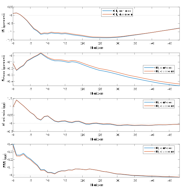
IP and prices are approximate percent responses; the short rate and excess bond premium are percentage-point responses. Both specifications use the same twelve-lag VAR and the same 240 instrument months. Differences come from centering the identifying moments. These are point estimates without confidence bands; the original bootstrap files are not presented as newly verified uncertainty estimates.
The centered impact vector is approximately (0.1172,-0.1230,1,0.3991)'. Its small positive IP impact is not a coding failure: this identification imposes no contemporaneous zero or negative sign on IP. Interpret the full path and the assumptions, not whether an unrestricted coefficient matches a preferred sign.
6 A variance normalization
For a one-standard-deviation orthogonal shock, let S satisfy SS'=\Sigma_u. The policy-unit direction can be rescaled as
b=\frac{s}{\sqrt{s'\Sigma_u^{-1}s}} =\frac{s}{\|S^{-1}s\|}.
This makes q=S^{-1}b a unit vector, so it can be completed to an orthogonal rotation. The identified shock’s forecast-error variance share through response horizon h is
\frac{\sum_{r=0}^{h}(e_i'C_rb)^2} {\sum_{r=0}^{h}e_i'C_r\Sigma_u C_r'e_i}.
The numerator must use b, not the policy-unit vector s. At economic horizon zero, this is the share of the one-step innovation variance. The code stores this targeted-shock share separately from the policy-unit impulse responses. It does not assign the remainder to named economic shocks.
7 Reading the implementation
replicate.m reads the two pinned files, checks monthly dates, fits the reduced form, and calls tsma.ident.proxy for centered GK, classroom GK, and centered MAR moments. The returned objects retain the overlap calendar, the exact instrument and innovations used, moments, first-stage residuals, and normalizations. No original helper is needed for ordinary execution.
verify_session05 is an optional private-source audit. It runs the source VAR and first-stage helper, forms the classroom second-stage coefficients, and compares every response over horizons 0-48. A close match of the uncentered calculation verifies compatibility. It does not erase the documented difference between centered and uncentered specifications.
8 Exercises
Recovering a direction
Suppose the covariance vector between four VAR innovations and a valid instrument is m=(-0.2,-0.1,0.4,0.12)', with the third variable as policy indicator. Find the one-unit policy impact vector. What happens if the instrument is multiplied by -100?
Hint: The normalization divides every entry by the policy entry.
The two-stage algebra
Derive the no-intercept two-stage coefficient using a scalar instrument z, policy residual u_p, and another residual u_q. Then explain which variables must be centered to include an intercept.
Hint: Write \widehat u_p=az and substitute a=z'u_p/(z'z).
A missing month
A VAR has residuals for January-April, while the instrument is observed in January, March, and April with values (1,0,-1). List the identifying sample. Should March’s observed zero be removed? What happens if the code uses the first three residual rows instead of a dated match?
Hint: Distinguish an unobserved value from an observed zero.
Unit variance and weak normalization
Let \Sigma_u=\operatorname{diag}(4,1) and s=(2,1)'. Find the unit-variance impact vector and each variable’s impact FEVD share. Separately, if m=(0.2,0.001)' and policy is variable two, calculate the effect of changing the policy covariance to 0.002 while keeping the first entry fixed. Does the normalization’s numerical existence establish strong identification?
Hint: Use s'\Sigma_u^{-1}s for variance scaling and compare two ratios.