Sign and narrative restrictions
Session 04 · Lecture notes
Which monetary-policy responses remain possible when identification specifies directions rather than contemporaneous zeros? These notes construct the admissible rotations of a quarterly VAR, distinguish a joint structural model from pointwise summaries, and explain what a dated narrative restriction adds. The application revisits the BSE sign-restriction exercise using GDP, a price index, and the federal funds rate. Prerequisites: Sessions 01-03 and QR decomposition.
1 The identifying question
A recursive VAR requires some variables not to respond immediately to a particular innovation. A sign-restricted VAR asks a different question: which structural systems are consistent with specified directions of response? Several systems can satisfy those restrictions. The result is then a set of possible models, not one uniquely identified monetary-policy shock.
I retain the classroom’s quarterly application and make its acceptance rule explicit. The variables are log real GDP, log PCE prices, and the federal funds rate. The input column is PCEPI, a price index, despite a classroom comment describing consumption. Calling this series real consumption would change the meaning of the supply and monetary restrictions.
The source sample runs from 1959Q1 to 2021Q3. The incomplete final row is excluded by its date. GDP and prices remain in natural logs during estimation; their plotted responses are multiplied by 100. The interest rate is already in percentage points. A log response of 0.01 is approximately one percent; a rate response of 0.01 is one basis point.
2 Observational equivalence
Write the reduced form as
y_t=c+\sum_{\ell=1}^{p}A_\ell y_{t-\ell}+u_t, \qquad E(u_tu_t')=\Sigma_u.
Its moving-average matrices satisfy C_0=I and C_h=\sum_{\ell=1}^{\min(p,h)}A_\ell C_{h-\ell}. Suppose u_t=B\varepsilon_t, with E(\varepsilon_t\varepsilon_t')=I. Then BB'=\Sigma_u. If S is a lower Cholesky factor of \Sigma_u, every B=SQ with QQ'=I satisfies the covariance restriction:
(SQ)(SQ)'=SQQ'S'=SS'=\Sigma_u.
The Cholesky factor is a convenient starting point here, not the final economic identification. The response of variable i to shock j at horizon h is e_i'C_hSq_j. A different admissible column q_j generally changes that response without changing the fitted reduced-form VAR.
The rotation approach follows Rubio-Ramírez et al. (2010). Its identifying content is in the restrictions, not in a particular random-number seed. The seed makes a finite numerical approximation reproducible; it does not narrow the population identified set.
3 The classroom restrictions
The baseline applies the following signs at every horizon from zero through four. A blank entry means unrestricted, not zero.
| Response | Supply | Demand | Monetary contraction |
|---|---|---|---|
| GDP | + | + | |
| Prices | - | + | - |
| Federal funds rate | + | + |
This is the classroom’s three-shock specification. Its earlier one-shock illustration also restricts GDP to fall on impact; that additional GDP sign is not imposed on the monetary column above. The array in config.m has variables in rows and shocks in columns, the transpose of the original classroom restriction table. Its numerical horizons are economic horizons; the implementation adds one only when indexing MATLAB arrays.
For any shock, all active signs must hold jointly across variables and horizons. If every active sign is reversed, multiplying that column of Q by -1 repairs its orientation. If only some are reversed, the candidate must be rejected. Reversing a separate horizon would no longer describe one shock. When several columns are named, they must belong to the same orthogonal matrix; choosing a satisfactory column independently for each shock can destroy their orthogonality.
4 Sampling the admissible set
For each candidate, draw an n\times n matrix of independent standard normal entries and calculate its QR decomposition. Adjust the columns of Q so that the diagonal of R is positive. This removes the sign convention left arbitrary by a QR implementation. Apply the joint restrictions and retain the complete matrix only if they all pass.
The revised sampler has an explicit attempt cap. If the cap is reached, it raises an error rather than treating an unfilled block of zeros as an accepted response. A local RandStream leaves the user’s global random generator untouched. Both attempted and retained counts are saved.
% Check all restricted variables and horizons under one common shock orientation.
function direction = sign_orientation(response, signs)
% Check that every response row has one declared sign.
assert(size(response, 1) == numel(signs) && all(isfinite(response(:))), 'tsma:Signs', 'Response rows and signs must agree.');
% Zero means unrestricted, so exclude those rows from the acceptance criterion.
active = signs(:) ~= 0;
% Multiplication converts every required sign to a nonnegative restriction.
products = response(active, :) .* signs(active);
% No restrictions, or all satisfied restrictions, preserve the original orientation.
if all(products(:) >= 0)
    % A positive orientation leaves this column of Q unchanged.
    direction = 1;
% A fully reversed path can be repaired with one common sign reversal.
elseif all(products(:) <= 0)
    % Reversing the shock must reverse every horizon simultaneously.
    direction = -1;
% Mixed signs violate at least one condition in either orientation.
else
    % Zero tells the caller to reject this whole system.
    direction = 0;
% Finish the three-way classification.
end
% Return orientation without changing the supplied responses.
end
The source AIC selects six lags. Its criterion compares different effective samples across candidates and uses the original observation count in the covariance divisor and penalty. I preserve that convention for this replication; Session 01 discusses why a common candidate sample is often preferable for a new model-selection exercise. The selected model has 245 residual quarters. With seed 12345, 250 complete systems are retained from 5,551 attempted rotations, an acceptance rate of about 4.50 percent.
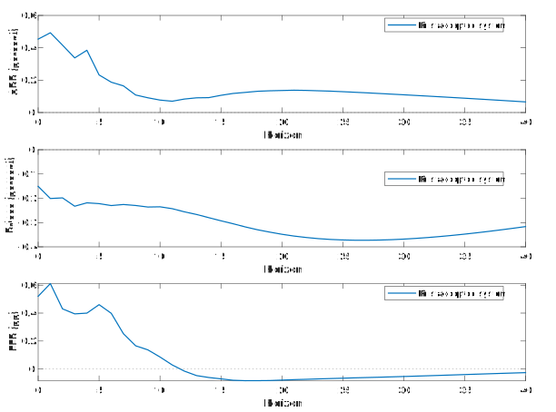
The figure shows one actual accepted system, conditional on the fitted reduced-form coefficients. Restrictions cover horizons 0-4. No restriction is placed on this monetary column’s GDP response. The shock has unit structural variance; it is not normalized to a one-percentage-point rate increase. The figure is not a confidence interval or a preferred economic model.
5 What the summaries mean
The saved array contains every variable, shock, horizon, and retained model. The 16th, 50th, and 84th pointwise empirical percentiles are also available, using order-statistic indices declared in the code. These summarize the sampled identification set conditional on one estimated reduced form. They do not incorporate sampling uncertainty in A_\ell or \Sigma_u.
A curve made from separate marginal medians need not correspond to any one admissible Q. It should not be used to recover a structural shock sequence, perform a historical decomposition, or calculate a coherent joint counterfactual. Those operations require a retained structural model. The distinction between model uncertainty and conventional inference is central to Fry and Pagan (2011). Drawing more rotations improves numerical coverage under the chosen rotation measure; it does not create a frequentist confidence level. Nor is a uniform measure on rotations economically uninformative in every parameterization.
6 Narrative information
A dated narrative restriction concerns a realized shock rather than an impulse response. For a candidate B=SQ, the realized structural innovation at date t^* is
\varepsilon_{t^*}=B^{-1}u_{t^*}.
If historical evidence supports a contractionary monetary shock at that date, an additional restriction is \varepsilon_{j,t^*}\geq0 under the chosen contractionary orientation. The code supports this extra filter through a residual-row index, a shock index, and an assumed sign. It does not activate an unsupported historical claim in the empirical baseline. The row must be matched to model.periods, because lag trimming shifts residual rows relative to the raw data.
This should not be confused with treating a constructed narrative series as an observed exogenous shock, as in the course’s narrative VAR-X discussion. Nor is it equivalent to using that series as a noisy external instrument. The latter approach requires relevance and exclusion restrictions and is the subject of Session 05. Historical evidence, a shock proxy, and a response-sign assumption supply different pieces of identification.
7 Reading the replication
Start with config.m, then follow replicate.m through dated import, lag selection, estimation, and rotation. The reusable sampler is tsma.ident.rotations; sign_orientation contains the entire acceptance logic for one column. verify_session04 compares coefficients, residuals, and the Wold recursion with the privately supplied original helpers, then passes every retained system through the original sign checker.
The numerical comparison does not require random draws from the original toolbox-dependent mvnrnd routine to have the same stream. It checks the estimated model and acceptance conditions themselves. The original files remain unchanged and are not included in the download.
8 Exercises
Orthogonal rotations
Let S=\begin{pmatrix}2&0\\1&1\end{pmatrix} and Q=\begin{pmatrix}0&-1\\1&0\end{pmatrix}. Calculate B=SQ and verify its covariance. Which economic restrictions, if any, follow merely from this calculation?
Hint: Compute QQ' before multiplying the impact matrices.
A joint sign test
For a supply shock, GDP must rise and prices must fall at horizons zero and one. Consider responses R_1=\begin{pmatrix}1&2\\-1&-3\end{pmatrix}, R_2=-R_1, and R_3=\begin{pmatrix}1&-2\\-1&3\end{pmatrix}. Classify each as accepted, accepted after reversal, or rejected. Explain why reversing one horizon of R_3 is invalid.
Hint: A column of Q fixes the shock’s orientation at every horizon.
Combining models
With \Sigma_u=I_2, let B_1=I_2 and B_2=\begin{pmatrix}0&-1\\1&0\end{pmatrix}. Does the entrywise average \bar B=(B_1+B_2)/2 reproduce \Sigma_u? What does this imply for combining pointwise summaries into a structural model?
Hint: The covariance restriction is quadratic rather than linear in B.
A dated restriction
Take B=\begin{pmatrix}1&0\\1&2\end{pmatrix} and a dated reduced-form innovation u_{t^*}=(1,-1)'. Recover the structural shocks. Does the model satisfy an assumption that the second shock was positive? What changes if the second column of B is reversed?
Hint: Solve two equations; do not calculate a matrix inverse explicitly.