Impulse responses and decompositions

Session 03 · Lecture notes

Abstract

This session follows a monetary policy innovation through an estimated VAR, quantifies pointwise uncertainty with a residual bootstrap, and decomposes forecast-error variances and observed histories. The implementation makes the horizon convention and initial-condition baseline explicit. Prerequisites: Sessions 01 and 02, conditional expectations, and variance.

Lecture PDF · Practicum · Worked solutions · Code package

1 Following a policy innovation

A response plot, a variance share, and a historical contribution all use the same estimated moving-average coefficients. They nevertheless answer different questions. The response plot describes an experiment. A variance share attributes uncertainty before future shocks occur. A historical contribution uses the shocks that were actually inferred from the sample.

The application follows the FEVD and historical-decomposition practical session (Boss 2024; Gambetti 2024). I retain its monthly data, VAR(3), variable order, and fifty-basis-point monetary experiment. I make the initial-condition component visible and replace the classroom two-stage bias-corrected bootstrap with a simpler, fully specified residual bootstrap. The new intervals are not a numerical replication of the source’s bias-corrected bands.

2 The horizon convention

Let u_t=B\varepsilon_t, with mutually orthogonal unit-variance shocks. The response at horizon h is

\Theta_h=C_hB,\qquad C_0=I,\qquad C_h=\sum_{j=1}^{\min(p,h)}A_jC_{h-j}.

The impact response is \Theta_0=B. In MATLAB, slice one represents h=0; slice 49 represents month 48. The following function propagates an arbitrary impact matrix and allows a single shock column as well as a square system.

% Propagate the columns of impact matrix B through a finite-order VAR.
function response = irf(A,B,H)
% Read the dimension of each response and the number of lag matrices.
[n,~,p] = size(A);
% Validate A through the same square-matrix check used in the stability routine.
tsma.var.companion(A);
% B may contain a subset of shocks, but every column must affect n variables.
assert(size(B,1)==n && all(isfinite(B),'all'), 'tsma:Dimensions', 'B must have n finite rows.');
% H denotes the last horizon, so the output has H+1 slices including impact.
assert(isscalar(H) && isfinite(H) && H>=0 && H==fix(H), 'tsma:Horizon', 'H must be a finite nonnegative integer.');
% Preallocate response variable by shock by horizon.
response = zeros(n,size(B,2),H+1);
% At horizon zero a unit structural innovation has immediate effect B.
response(:,:,1) = B;
% Recursively propagate each future horizon from already computed responses.
for horizon = 1:H
    % Only lags no longer than the elapsed horizon have nonzero past responses.
    for lag = 1:min(p,horizon)
        % MATLAB slice horizon-lag+1 represents economic horizon horizon-lag.
        response(:,:,horizon+1) = response(:,:,horizon+1) + A(:,:,lag)*response(:,:,horizon-lag+1);
    % End contributions from the available autoregressive lags.
    end
% End propagation through the requested horizon.
end
% Return all responses, retaining the impact slice even when H is zero.
end

The recursion permits a useful independent check. Form the companion matrix F and compare C_h with the first n rows and columns of F^h for every horizon. Agreement at impact alone would miss a transpose or lag-order error.

For the plotted policy response, multiply column four by 0.5/b_{44}. The funds-rate impact is then .5 percentage points. Sum the production and CPI growth responses across horizons to get their level effects. Do not cumulate unemployment, the rate, or NFCI, which already enter the model in levels. The level response at month 12 includes thirteen growth responses: impact through month 12.

3 Pointwise bootstrap intervals

The coefficients and covariance matrix are estimated, so the response path is uncertain. The residual bootstrap asks how the estimator behaves in pseudo-samples drawn from the fitted model. Here is the implemented algorithm:

1. Fit the original VAR and center its vector residuals. Multiply them by \sqrt{T/(T-k)} so their empirical covariance has the fitted degrees-of-freedom scale.
2. Keep the first p observed vectors as the initial history. Draw entire residual rows independently with replacement and simulate the remaining observations recursively. Sampling columns independently would destroy contemporaneous cross-equation dependence.
3. Re-estimate the VAR, recompute its Cholesky factor, normalize the policy shock, and construct the cumulative production and price responses.
4. Repeat 500 times with a private random stream seeded at 202403. Take the empirical .16 and .84 quantiles at each variable and horizon.

The empirical quantile is the sorted observation at index \lceil qB\rceil, where B=500 denotes the number of replications. Thus the interval endpoints use order statistics 80 and 420. The complete response array, coefficient draws, and companion-root moduli are saved. No draw is silently rejected for an unstable estimated root; this avoids conditioning the reference distribution on a stability screen.

The procedure assumes a well-specified constant-parameter VAR and independently resampleable, homoskedastic vector innovations. Conditional heteroskedasticity, serially dependent residuals, or major structural changes would motivate a different resampling scheme and a revised empirical model. The bootstrap does not repair a false identifying restriction.

Figure 1: Responses to a fifty-basis-point monetary innovation with pointwise 68 percent residual-bootstrap intervals.

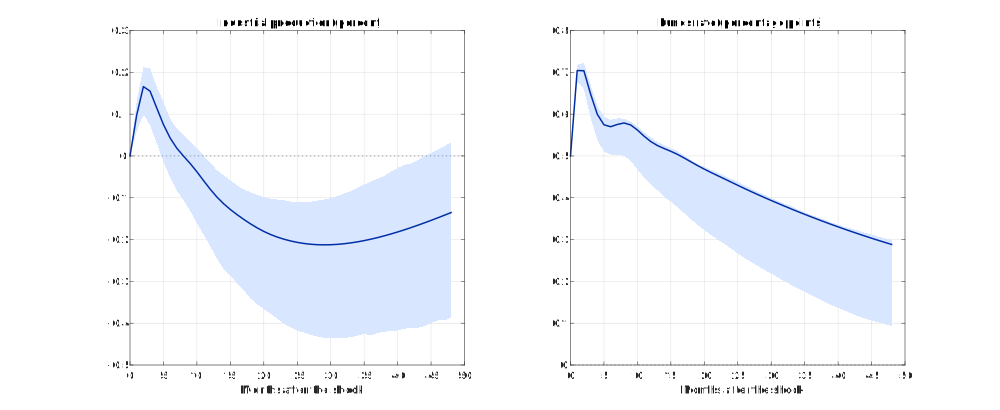
Production is a percent log-level response; the funds rate is in percentage points. The bootstrap conditions on the initial three observations and does not apply the classroom bias correction. The impact interval for the policy rate collapses to .5 by normalization, not because impact uncertainty was estimated to be zero.

The tested run retained all 500 draws; none had a companion root on or outside the unit circle. These are pointwise intervals. A 68 percent interval at each horizon does not imply that the entire true response curve lies inside the shaded region with 68 percent probability. Five hundred draws also leave Monte Carlo variation in the endpoints. Increasing the draw count is a numerical sensitivity check, not a new identification argument.

4 Forecast-error variance shares

For an H-step forecast made at t, future shocks contribute

y_{t+H}-E_t y_{t+H}=\sum_{j=0}^{H-1}\Theta_j\varepsilon_{t+H-j}.

Orthogonality makes the variance a sum of squared responses. The share of shock s in variable i’s forecast error is

\omega_{is}(H)= \frac{\sum_{j=0}^{H-1}\Theta_{is,j}^{\,2}} {\sum_{r=1}^{n}\sum_{j=0}^{H-1}\Theta_{ir,j}^{\,2}}.

The one-step variance uses only \Theta_0. Hence an IRF array with horizons 0 through 48 supplies FEVD horizons 1 through 49. Calling its final slice a “48-step FEVD” would be off by one.

For production and the price level, replace growth responses \Theta_j by their cumulative sums before squaring. Squaring a growth response and then cumulating does not produce the same object. The other modeled variables already enter in levels.

Use responses to unit-variance shocks for all columns. A column normalized to fifty basis points has a different variance scale; replacing only that column in the FEVD calculation changes the shares. If shock variances are not one, their variance weights must be included explicitly.

In this data, policy accounts for about 96.69 percent of the funds-rate one-step forecast error variance, 77.36 percent at 13 steps, and 69.03 percent at 49 steps. For the production level the corresponding shares are zero, about .57 percent, and 2.19 percent. The impact zero follows from the recursive restriction, not from an estimated absence of monetary effects at every horizon. Each variable-horizon row sums to one by construction; a zero total variance is undefined and triggers an error.

5 Historical accounting

Let \tau_0 be the first fitted residual date. The finite-sample contribution of shock s to variable i at date t\geq\tau_0 is

d_{is,t}=\sum_{\tau=\tau_0}^{t} \Theta_{is,t-\tau}\widehat\varepsilon_{s,\tau}, \qquad \widehat\varepsilon_t=B^{-1}\widehat u_t.

The code obtains the shocks with a linear solve rather than an explicit inverse. It computes the contribution sequences by convolution and keeps the exact residual dates.

The contributions alone generally do not add to the observed data. Define a_t as the VAR path that starts from the observed initial p vectors, retains the intercept, and receives zero later innovations. Then

y_{i,t}=a_{i,t}+\sum_{s=1}^n d_{is,t}.

The baseline includes initial conditions and the intercept, not an additional structural shock. In the tested sample the maximum reconstruction discrepancy is approximately 3.3\times10^{-14}. That is an accounting check on units, orientation, and date alignment.

A shock contribution can be negative. It is a signed additive term, not a variance share, and there is no adding-up-to-one rule. Contributions to production growth can be cumulated if the question concerns a normalized production-level path; the baseline and initial level must then be treated consistently. This replication reports the decomposition of the modeled variables, not a relabeled decomposition of their raw levels.

Finally, a historical decomposition depends on the entire estimated model. It is not an experimental estimate of the outcome that would have occurred under a different monetary policy rule. Holding the estimated dynamics fixed while removing inferred shocks is a conditional accounting exercise; a policy regime change may alter those dynamics.

6 Verification and files

The shared tests compare lag recursion with companion powers, check an FEVD by hand, and reconstruct a small sample from its initial state and shocks. The empirical replication checks the same adding-up identities and saves every bootstrap draw. The monthly reduced form and Wold responses also match the fingerprinted classroom helpers across all twenty candidate lag orders.

The entrypoint writes the full result to the session’s outputs directory. The practicum shows how to read the array dimensions before slicing a particular response. It also checks that the normalized impact appears in every bootstrap draw, which is a direct test of the implemented experiment.

7 Exercises

Impact and one-step uncertainty

Let A=\operatorname{diag}(.5,.2) and B=\begin{pmatrix}1&0\\1&2\end{pmatrix}. Compute \Theta_0 and \Theta_1. Then calculate the two-step forecast-error variance shares for variable two. Why does the two-step calculation not use \Theta_2?

Hint: List the two future innovations that remain unknown at the forecast origin.

Reconstructing a history

For y_t=1+.5y_{t-1}+\varepsilon_t, take y_0=2 and innovations (\varepsilon_1,\varepsilon_2,\varepsilon_3)=(1,-2,0). Calculate the observed path, the zero-future-shock baseline, and the shock contribution at each date. Verify reconstruction.

Hint: The effect of an innovation is multiplied by .5 each subsequent period.

Reading a bootstrap interval

With 500 sorted response draws, the empirical quantile rule is x_{(\lceil500q\rceil)}. Which draws form the central 68 percent interval? If each of two independent horizon intervals covers its target with probability .68, what is the probability both cover? Why is that calculation not a formula for actual VAR simultaneous coverage?

Hint: Distinguish Monte Carlo quantiles, pointwise coverage, and dependence between horizons.

Growth and levels

For one outcome and two orthogonal unit-variance shocks, growth responses are (1,1) on impact and (-1,1) one period later. Compute the two-step FEVD for growth and for the outcome’s log level.

Hint: Cumulate the growth responses separately for each shock before squaring them for the level calculation.

References

Boss, Konstantin. 2024. “Time Series Models for Macroeconometric Analysis: Practical Materials.” Unpublished manuscript.

Gambetti, Luca. 2024. “Time Series Models for Macroeconometric Analysis: Lecture Notes.” Unpublished manuscript.