Structural identification
Session 02 · Lecture notes
Reduced-form forecast errors need identifying assumptions before they can be interpreted as economic shocks. I work through recursive monetary identification and long-run technology restrictions using the course data. The calculations separate shock scale, variable ordering, and the horizon over which a restriction is imposed. Prerequisites: Session 01, covariance matrices, and Cholesky factorization.
1 Forecast errors and economic shocks
A funds-rate surprise can accompany new information about inflation, an independent policy decision, or a financial disturbance. A VAR residual mixes those sources of variation. Calling the fourth residual a monetary shock would skip the central identifying problem.
I use two course applications to distinguish restrictions on impact from restrictions in the long run (Boss 2024; Gambetti 2024). The first retains the five monthly variables from Session 01. The second uses productivity and hours growth from the classroom Fernald workbook. Neither exercise identifies a shock merely because its response looks familiar.
Write the reduced-form error as
u_t=B\varepsilon_t,\qquad E(\varepsilon_t\varepsilon_t')=I,\qquad \Sigma=BB'.
There are n^2 entries in B but only n(n+1)/2 distinct covariance moments. A nonsingular system therefore needs another n(n-1)/2 restrictions to select a particular orthogonalization, together with sign and labeling conventions. For any orthogonal Q, (BQ)(BQ)'=\Sigma. Matching the covariance alone does not distinguish B from BQ.
This representation also assumes that the economically relevant shocks are recoverable from the VAR’s information set. If agents observe news that the econometrician does not, the estimated innovations need not span the desired structural shocks. Adding a zero restriction cannot by itself fix that information problem.
2 Recursive monetary identification
Order the monthly variables as production growth, inflation, unemployment, the funds rate, and NFCI. A lower-triangular Cholesky factor has the pattern
B=\begin{pmatrix} b_{11}&0&0&0&0\\ b_{21}&b_{22}&0&0&0\\ b_{31}&b_{32}&b_{33}&0&0\\ b_{41}&b_{42}&b_{43}&b_{44}&0\\ b_{51}&b_{52}&b_{53}&b_{54}&b_{55} \end{pmatrix},\qquad b_{jj}>0.
The monetary shock is column four. Production, prices, and unemployment do not respond to that shock within the month; NFCI may respond immediately. The funds rate may respond within the month to the first three shocks, but not to the fifth financial-conditions shock. These are timing assumptions about the monthly observations, not conclusions estimated from the zeros.
With C_0=I and the Wold recursion from Session 01, the structural response matrix is \Theta_h=C_hB. A unit shock has variance one. Its funds-rate impact is b_{44} percentage points, which generally is not one percentage point.
For a fifty-basis-point policy experiment, use only
b^{MP}_{50}=B_{\cdot4}\frac{0.5}{b_{44}},\qquad \theta^{MP}_{h,50}=C_hb^{MP}_{50}.
The numerator is .5, not 50: the rate is recorded in percentage points. Do not rescale every column when the question concerns only shock four. Keep the unscaled B for shock recovery and variance decompositions.
Production and CPI enter in monthly log changes. Their cumulative responses through h are \sum_{j=0}^h\theta_j, approximately percent level differences. The rate and unemployment enter in levels, so their plotted responses are not cumulative. Summing a rate response measures a different object.
3 A long-run restriction
The quarterly application follows the classroom exercise motivated by Blanchard and Quah’s long-run identification and Galí’s technology analysis (Blanchard and Quah 1989; Galí 1999). Let y_t=(g^a_t,g^\ell_t)' contain annualized growth in labor productivity and hours. Assume that only shock one can have a permanent effect on productivity’s level. Then
D=C(1)B=\begin{pmatrix}d_{11}&0\\d_{21}&d_{22}\end{pmatrix}, \qquad d_{11},d_{22}>0,
where the exact multiplier for a stable VAR is
C(1)=\sum_{h=0}^{\infty}C_h= \left(I-\sum_{j=1}^p A_j\right)^{-1}.
The zero is in D, not necessarily in B. A nontechnology shock can move productivity immediately but must have zero cumulative long-run effect. The positive first diagonal entry defines a favorable technology shock.
Since DD'=C(1)\Sigma C(1)', construct its lower Cholesky factor and recover B=C(1)^{-1}D. The implementation uses linear solves and checks stability:
% Identify shocks by a lower-triangular infinite-horizon cumulative response.
function identified = long_run(model)
% A finite long-run multiplier requires a stable autoregression.
assert(max(abs(model.roots))<1, 'tsma:Stability', 'Long-run identification requires a stable VAR.');
% Construct the autoregressive polynomial at one, not a truncated sum of IRFs.
polynomial = eye(model.n)-sum(model.A,3);
% Reject a numerically singular long-run multiplier before factorization.
assert(rcond(polynomial)>1e-10, 'tsma:LongRun', 'Long-run multiplier is ill conditioned.');
% Solve for C(1) without explicitly forming an inverse.
identified.C = polynomial\eye(model.n);
% Factor the implied long-run covariance with positive diagonal normalization.
identified.longImpact = chol(identified.C*model.Sigma*identified.C','lower');
% Recover contemporaneous impacts consistent with those long-run restrictions.
identified.B = polynomial*identified.longImpact;
% Record reconstruction error for the identifying covariance identity.
identified.covarianceError = max(abs(identified.B*identified.B'-model.Sigma),[],'all');
% Return both impact and long-run effects so readers can check the restriction.
end
The economic assumption does not come from Cholesky algebra. A permanent productivity component could reflect omitted influences rather than pure technology. Near-unit roots also make the long-run multiplier sensitive to small coefficient changes. A numerically valid factorization is therefore necessary for this exercise, but not sufficient for a persuasive empirical interpretation.
4 The quarterly application
The classroom workbook has Fernald’s annualized quarterly growth rates (Fernald 2014). I select dates 1947 Q2 through 2022 Q4 by their labels, not row positions. The series are labor-productivity growth and hours growth for the business sector. This expands and changes the data relative to Galí’s published application. It is a replication of the course exercise, not the paper’s original sample or every published specification.
The archived AIC convention selects four lags. The model uses 299 dependent quarters and has maximum companion-root modulus about .6865. The exact impact matrix in the workbook’s annualized growth units is approximately
\widehat B= \begin{pmatrix} 2.6416&1.5516\\ -3.3834&3.7493 \end{pmatrix}.
A unit favorable technology shock raises annualized productivity growth and lowers annualized hours growth on impact in this fitted system. Converting to quarterly log levels requires a factor of one fourth:
\text{level response at }h=\frac14\sum_{j=0}^h\Theta_j.
Thus the impact log-level responses to technology are about .6604 percent for productivity and -.8459 percent for hours. Annualization is a unit conversion, not another identifying restriction.
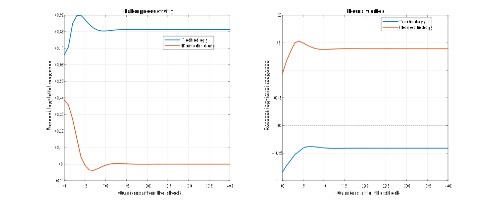
Responses to unit-variance shocks. Annualized quarterly growth responses are divided by four before cumulation. These are point estimates; the figure does not claim confidence coverage.
The original script approximates C(1) by summing responses through quarter 40. I retain that calculation separately. In this sample its impact matrix differs from the exact solution by about 5.0\times10^{-7} at most. The difference is small because the fitted system decays quickly. That numerical coincidence is not a justification for treating an arbitrary finite horizon as infinity in another dataset.
5 Restrictions that mix horizons
Some economic hypotheses impose a zero on impact and a different restriction on a cumulative response. They cannot generally be imposed by taking a Cholesky factor twice. Starting from any covariance factor P, write B=PQ. An impact zero for response i to shock j is e_i'Pq_j=0; a long-run zero is e_i'C(1)Pq_j=0. For a given shock, stack the relevant rows and seek a unit vector in their null space, subject to orthogonality to already selected shocks.
Too many independent restrictions can leave no nonzero direction; too few leave a set of admissible directions. The worked exercise shows this in two dimensions. Session 04 develops rotations when inequalities, rather than a fully identifying set of equalities, define admissibility.
6 What the checks establish
The monthly application uses the same VAR(3) as the classroom benchmark. For the quarterly application, an optional comparison runs the original fingerprinted Galí-family VAR and Wold helpers for all four lag orders. Covariance reconstruction checks verify \widehat B\widehat B'=\widehat\Sigma; the long-run check verifies (C(1)\widehat B)_{12}=0.
These algebraic and numerical checks locate transcription or implementation errors. They do not test whether the recursive ordering is true, whether the identified permanent component is technology, or whether the omitted information set is harmless. Those questions belong in the interpretation, not in a silent normalization step.
7 Exercises
A recursive shock
Let \Sigma=\begin{pmatrix}4&2\\2&5\end{pmatrix} and order variable one before variable two. Derive the lower-triangular factor with positive diagonal. Normalize the second shock to an own-variable impact of .5. What happens to covariance reconstruction if that normalized column replaces the original column while both shocks are still assumed to have variance one?
Hint: Begin with b_{11}^2=4, then use the covariance equation.
The infinite-horizon zero
Let A=\begin{pmatrix}.5&0\\0&.25\end{pmatrix} and retain the same \Sigma. Compute C(1), its implied long-run covariance, the lower factor D, and B=C(1)^{-1}D. Check the long-run zero directly.
Hint: The inverse of a diagonal matrix is diagonal, so this example can be completed without a numerical solver.
Conflicting restrictions
In a bivariate model with P=I, require the first shock to have zero impact on variable one. Also require zero long-run effect on variable two, where C(1)=\begin{pmatrix}2&1\\1&2\end{pmatrix}. Is there a unit vector q_1 satisfying both restrictions? Explain why merely counting two requested restrictions does not establish identification.
Hint: Write the two row equations before imposing q_1'q_1=1.
Annualized growth
An annualized quarterly growth response is 4 on impact, 2 one quarter later, and 0 thereafter. Compute the log-level response at horizons zero, one, and ten. What would the answer be if those numbers were already quarterly, nonannualized log growth?
Hint: Convert the growth rate’s units before cumulating.