Reduced-form VARs
Session 01 · Lecture notes
A monthly system for industrial production, inflation, unemployment, the federal funds rate, and financial conditions introduces VAR estimation. I make transformations and the calendar explicit, compare lag criteria on a common sample, and use the estimated system to construct forecasts. Prerequisites: least squares, matrix multiplication, and logarithms.
1 A monthly system
How much does the recent history of activity, prices, and financial conditions tell us about next month’s economy? A vector autoregression answers a prediction question first. Its residuals are forecast errors, not yet monetary policy shocks. Identification comes in the next session.
The application follows Boss’s first practical session and the VAR discussion in Gambetti’s notes (Boss 2024; Gambetti 2024). I retain the archived data vintage and variable order. My main changes concern the calendar, the least-squares calculation, and the sample used to compare lag orders.
Let the five-by-one monthly observation be
y_t=(g^{IP}_t,\pi_t,u_t,i_t,f_t)',\qquad g^{IP}_t=100(\log IP_t-\log IP_{t-1}),\quad \pi_t=100(\log CPI_t-\log CPI_{t-1}).
Production growth and inflation are monthly log-percent changes. They are not annualized. Unemployment and the funds rate remain in percentage points; NFCI remains an index. Differencing an already differenced rate, or multiplying the interest rate by 100, would change the question without changing the code’s ability to run. Named columns and unit checks prevent those mistakes.
The CSV contains January 1971 through January 2024. The first month supplies lagged index levels. The final month has missing production and CPI values. The transformed window is February 1971 through December 2023, 635 observations. The importer preserves missing values and records integer month identifiers. It never treats the next available row as the next month when a calendar month is absent.
2 The regression
A VAR with an intercept and p lags is
y_t=c+A_1y_{t-1}+\cdots+A_py_{t-p}+u_t, \qquad E(u_t\mid\mathcal F_{t-1})=0.
Each equation uses the same regressors. Stack the T usable observations as Y=X\Gamma+U, where X has k=1+np columns and \Gamma is k\times n. The first row of \Gamma is c'. The next n rows are A_1', not A_1. That transpose matters when regression output becomes a dynamic system.
For a two-variable VAR(2), one design row is
x_t'=(1,y_{1,t-1},y_{2,t-1},y_{1,t-2},y_{2,t-2}).
OLS gives \widehat\Gamma=(X'X)^{-1}X'Y. This is a mathematical formula, not an instruction to calculate an inverse. The implementation factors X=QR and solves R\widehat\Gamma=Q'Y. It rejects rank-deficient designs and keeps the full design, coefficients, residuals, and usable dates.
With the same regressors in every equation, GLS exploiting contemporaneous cross-equation correlation does not change these coefficient estimates. Under homoskedastic, serially uncorrelated innovations, the conventional covariance estimators are
\widehat\Sigma=\frac{\widehat U'\widehat U}{T-k},\qquad \widehat{\operatorname{Var}}\{\operatorname{vec}(\widehat\Gamma)\} =\widehat\Sigma\otimes(X'X)^{-1}.
Here T already excludes unusable lag rows. Do not subtract p again. Vectorization stacks one equation’s coefficient column after another. The covariance formula is not HAC: residual serial correlation would undermine the maintained finite-order specification and this conventional inference. OLS in a dynamic model also has finite-sample bias; the degrees-of-freedom correction to \widehat\Sigma does not remove coefficient bias.
3 Choosing the lag order
Adding lags improves in-sample fit but consumes n^2 coefficients per lag. For each candidate, use the Gaussian fit term \log|\widehat\Sigma_{ML}|, with \widehat\Sigma_{ML}=\widehat U'\widehat U/T. Apart from constants common to all candidates, the criteria are
\begin{aligned} AIC(p)&=\log|\widehat\Sigma_{ML,p}|+2nk_p/T,\\ BIC(p)&=\log|\widehat\Sigma_{ML,p}|+\log(T)nk_p/T,\\ HQ(p)&=\log|\widehat\Sigma_{ML,p}|+2\log\log(T)nk_p/T. \end{aligned}
I compare candidates p=1,\ldots,20 on the same 615 dependent dates. The extra initial observations needed by shorter models are excluded from their comparison fit. After selecting a lag length, I refit that model on its full available sample. Information criteria do not establish causal identification and a BIC minimum does not prove white-noise residuals.
The classroom helper changes the dependent sample with p and divides each residual product by the original 635 observations. I preserve that calculation as classroom mode, rather than quietly substituting it for the common-sample criterion. The two rules yield:
| Comparison | AIC | BIC | HQ |
|---|---|---|---|
| Common dependent sample | 10 | 3 | 3 |
| Classroom convention | 14 | 3 | 6 |
Both BIC choices happen to be three in this vintage. The different AIC and HQ choices show why sample conventions belong in a replication record.
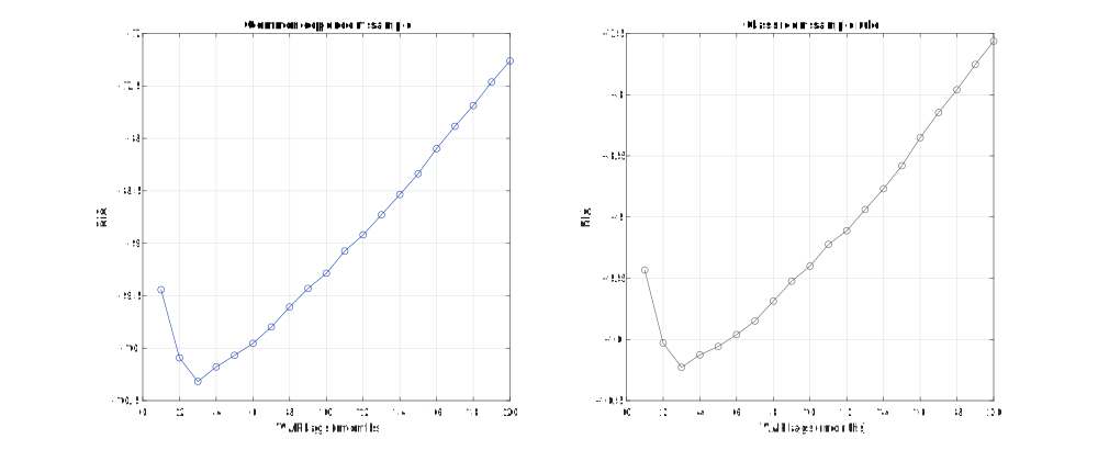
The score levels in the two panels should not be compared as likelihoods of the same observations. Generated by the publication function from the fingerprinted practical-session data.
4 Stability and propagation
Stack s_t=(y_t',y_{t-1}',\ldots,y_{t-p+1}')'. The companion representation is
s_t=\widetilde c+Fs_{t-1}+Ju_t,\qquad C_h=J'F^hJ,
where J inserts an n-vector in the first block of the np-vector state. All eigenvalues of F must have modulus below one for the stable infinite moving-average representation. A coefficient larger than one in one equation is not, by itself, the stability test. Conversely, individually small coefficients need not imply a stable multivariate system.
The fitted VAR(3) uses 632 observations from May 1971 through December 2023. Its largest companion-root modulus is about 0.9854: stable, but persistent. This is a property of the fitted constant-parameter model, not evidence that monetary transmission was unchanged over five decades.
5 Forecasts
Set future innovations to their conditional mean of zero. For one step,
\widehat y_{T+1\mid T}=\widehat c+ \sum_{j=1}^{p}\widehat A_jy_{T+1-j}.
At two steps, replace the unavailable y_{T+1} by the one-step forecast. Continue recursively, preserving observed lags until each is replaced by a prediction. The following is the actual forecasting function.
% Compute conditional mean forecasts, holding future innovations at zero.
function predicted = forecast(model,history,H)
% Require p consecutive, complete observations ending at the forecast origin.
assert(size(history,1)>=model.p && size(history,2)==model.n && all(isfinite(history),'all'), 'tsma:History', 'Supply at least p complete history rows.');
% Permit impact-only requests to return an empty future-forecast matrix.
assert(isscalar(H) && isfinite(H) && H>=0 && H==fix(H), 'tsma:Horizon', 'H must be a finite nonnegative integer.');
% Keep the p most recent observations in chronological order.
state = history(end-model.p+1:end,:);
% Preallocate future observations in the same units as the fitted outcomes.
predicted = zeros(H,model.n);
% Feed previous predictions into the next forecast's lag vector.
for h = 1:H
    % The lag-major design is intercept, y_t, y_t-1, and so forth.
    regressor = [1,reshape(flipud(state)',1,[])];
    % Evaluate the fitted conditional mean with no future innovation.
    predicted(h,:) = regressor*model.beta;
    % Advance the state by one period, including the just-computed forecast.
    state = [state(2:end,:);predicted(h,:)];
% End the recursive forecast.
end
% Return horizon one in the first row, unlike IRFs whose first slice is impact.
end
The first forecast row is January 2024, not horizon zero. It gives approximately 0.0229 percent production growth and 0.2795 percent inflation, with unemployment at 3.7813 percent and the funds rate at 5.3278 percent. These are conditional means under a fitted historical model. The replication does not claim an out-of-sample accuracy result or a real-time forecast: it uses the archived vintage and has not scored predictions against a separately acquired evaluation sample. A proper evaluation would select lags inside each training window and distinguish revised data from the information available at the forecast date.
6 Reading the implementation
Start with the configuration, then the named importer, lag selector, and least-squares estimator. The entrypoint saves full model objects and CSV tables under the session’s outputs directory. The optional source comparison executes only five SHA-256-pinned classroom helpers from a user-supplied archive. Across all twenty lag orders, it compares every coefficient, residual, and Wold response through month 48. The largest discrepancy is below 6\times10^{-11}, against a declared 10^{-8} tolerance. This verifies the refactor under the source conventions; the common-sample criterion is a separately documented revision.
7 Exercises
The first design row
A bivariate series has observations (1,2), (3,1), (2,4), (5,3), and (4,6) at dates 1 through 5. Write X and Y for an intercept VAR(2). Can this system be estimated with positive residual degrees of freedom? Then remove date 3. Which dependent observations still have both required lags?
Hint: Count usable rows and coefficients per equation separately.
Two forecasts
For y_t=c+Ay_{t-1}+u_t, let c=(1,0)', A=\begin{pmatrix}0.5&0.2\\0&0.4\end{pmatrix}, and y_T=(2,5)'. Compute the one- and two-step conditional mean forecasts, the unconditional mean, and the stability roots. Why is a forecast not an impulse response?
Hint: An IRF holds the baseline fixed and tracks an innovation; a forecast also carries the intercept and observed state.
Comparing information criteria
Two bivariate VARs use a common sample of T=100. Their lag orders are one and two, and their covariance log determinants are -2 and -2.1. Compute AIC and BIC, counting the intercepts. What would become ambiguous if the larger model instead dropped ten additional dependent observations?
Hint: The coefficient counts across the system are n(1+np).